Low Overhead Program Monitoring and Profiling Naveen Kumar

Low Overhead Program Monitoring and Profiling Naveen Kumar, Bruce Childers Department of Computer Science University of Pittsburgh, Pennsylvania 15260 {naveen, childers}@cs. pitt. edu Mary Lou Soffa Department of Computer Science University of Virginia Charlottesville, Virginia 22904 soffa@virginia. edu 1

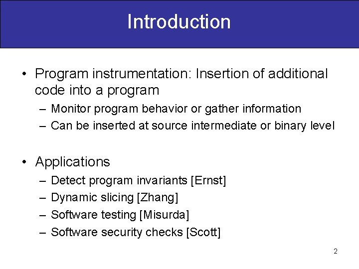
Introduction • Program instrumentation: Insertion of additional code into a program – Monitor program behavior or gather information – Can be inserted at source intermediate or binary level • Applications – – Detect program invariants [Ernst] Dynamic slicing [Zhang] Software testing [Misurda] Software security checks [Scott] 2

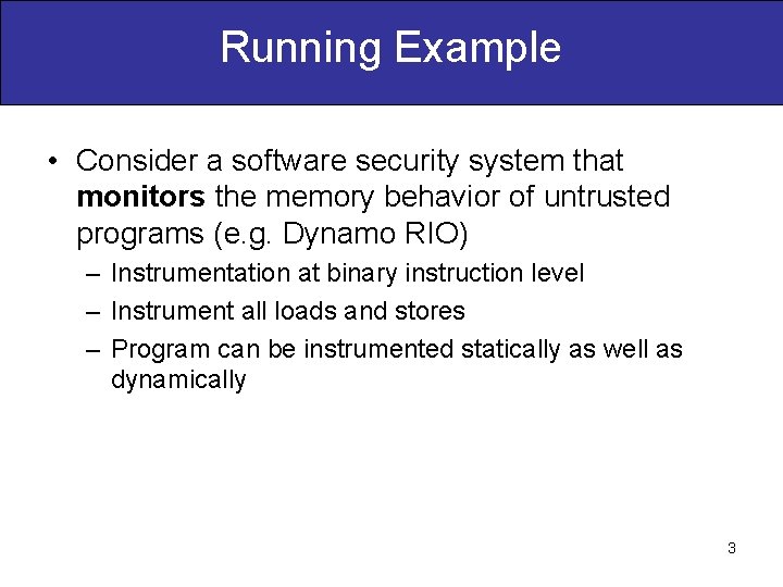
Running Example • Consider a software security system that monitors the memory behavior of untrusted programs (e. g. Dynamo RIO) – Instrumentation at binary instruction level – Instrument all loads and stores – Program can be instrumented statically as well as dynamically 3

Static instrumentation r[o 1] = r[o 1] << 10 r[o 1] = r[o 1] + 0 x 228 r[o 0] = r[o 2] << 0 x 14 r[l 4] = r[o 0] << 0 x 14 jmp probe 1 M[r[l 0 ]+ 0 x 10 ] = r[o 2] M[r[o 1] + 0 x 228 ] = r[o 0] jmp probe 2 r[i 4] = r[o 1] r[l 1] = r[o 0] jmp r[31] … M[r[l 0] + 0 x 20 ] = r[o 0] jmp probe 3 r[sp] = r[sp] -112 r[o 0] = r[o 0] << 10 r[o 1] = M[r[o 0] + 0 x 3 d 0 ] jmp probe 4 … … probe 1: call M[r[sp] secure(…) + -20 ] = r[l 0] save probe 2: call save_gp_regs call … secure(…) r[o 0] = M[r[sp] + 0 x 68 ] probe 3: r[o 0] = r[o 0] +0 x 10 call secure(…) secure r[o 1] = r[g 0] + 1 probe 4: call restore_gp_regs call secure(…) restore r[sp] = r[sp] + 124 M[r[l 0 ]+ 0 x 10 ] = r[o 2] jmp probe 1_ret Example from gzip. Instrumentation performed before execution starts 4

Dynamic instrumentation r[o 1] = r[o 1] << 10 r[o 1] = r[o 1] + 0 x 228 r[o 0] = r[o 2] << 0 x 14 r[l 4] = r[o 0] << 0 x 14 jmp probe 1 M[r[l 0 ]+ 0 x 10 ] = r[o 2] M[r[o 1] + 0 x 228 ] = r[o 0] jmp probe 2 r[i 4] = r[o 1] r[l 1] = r[o 0] jmp r[31] … M[r[l 0] + 0 x 20 ] = r[o 0] jmp probe 3 r[sp] = r[sp] -112 r[o 0] = r[o 0] << 10 r[o 1] = M[r[o 0] + 0 x 3 d 0 ] jmp probe 4 … … probe 1: call secure(…) probe 2: call secure(…) probe 3: call secure(…) probe 4: call secure(…) Instrumentation performed at run-time on code that executes 5 More powerful than static instrumentation, possibly less expensive

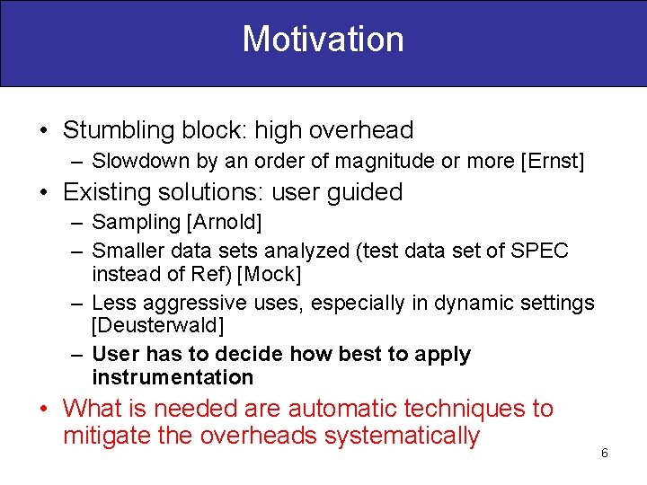
Motivation • Stumbling block: high overhead – Slowdown by an order of magnitude or more [Ernst] • Existing solutions: user guided – Sampling [Arnold] – Smaller data sets analyzed (test data set of SPEC instead of Ref) [Mock] – Less aggressive uses, especially in dynamic settings [Deusterwald] – User has to decide how best to apply instrumentation • What is needed are automatic techniques to mitigate the overheads systematically 6

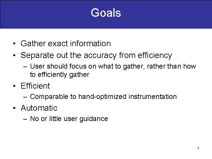
Goals • Gather exact information • Separate out the accuracy from efficiency – User should focus on what to gather, rather than how to efficiently gather • Efficient – Comparable to hand-optimized instrumentation • Automatic – No or little user guidance 7

Instrumentation Optimization • Costs associated with instrumentation – Dynamic probe count: Number of probes executed – Probe cost: Number of instructions in a probe – Payload cost: Frequency of invocation and cost of payload • Optimize instrumentation code to reduce costs – Dynamic probe coalescing – Partial context switches – Partial payload inlining 8

Base Instrumenter r[o 1] = r[o 1] << 10 r[o 1] = r[o 1] + 0 x 228 r[o 0] = r[o 2] << 0 x 14 r[l 4] = r[o 0] << 0 x 14 jmp probe 1 M[r[l 0 ]+ 0 x 10 ] = r[o 2] M[r[o 1] + 0 x 228 ] = r[o 0] jmp probe 2 r[i 4] = r[o 1] r[l 1] = r[o 0] jmp r[31] … M[r[l 0] + 0 x 20 ] = r[o 0] jmp probe 3 r[sp] = r[sp] -112 r[o 0] = r[o 0] << 10 r[o 1] = M[r[o 0] + 0 x 3 d 0 ] jmp probe 4 … … probe 1: call secure(…) probe 2: call secure(…) probe 3: call secure(…) probe 4: call secure(…) 9 Base instrumenter generates a list of Instrumentation Points

Dynamic Probe Coalescing r[o 1] = r[o 1] << 10 r[o 1] = r[o 1] + 0 x 228 r[o 0] = r[o 2] << 0 x 14 r[l 4] = r[o 0] << 0 x 14 jmp probe 1 M[r[l 0 ]+ 0 x 10 ] = r[o 2] jmp probe 2 probe 5 M[r[o 1] + 0 x 228 ] = r[o 0] r[i 4] = r[o 1] r[l 1] = r[o 0] jmp r[31] … M[r[l 0] + 0 x 20 ] = r[o 0] jmp probe 3 probe 6 r[sp] = r[sp] -112 r[o 0] = r[o 0] << 10 r[o 1] = M[r[o 0] + 0 x 3 d 0 ] jmp probe 4 … … probe 6: probe 5: probe 1: call secure(…) probe 2: call secure(…) probe 3: call secure(…) probe 4: call secure(…) 10

Partial Context Switch probe 6: call secure(…) M[r[sp] -20 ] = r[l 0] r[o 1] = r[o 1] << 10 r[o 1] = r[o 1] + 0 x 228 call secure(…) M[r[sp] -28 ] = r[o 1] r[o 0] = r[o 2] << 0 x 14 call savesecure(…) r[l 4] = r[o 0] << 0 x 14 call save_gp_regs M[r[l 0 ]+ 0 x 10 ] = r[o 2] M[r[o 1] + 0 x 228 ] = r[o 0] … effective address … r[i 4] = r[o 1] call secure r[l 1] = r[o 0] … effective address … jmp r[31] … call secure M[r[l 0] + 0 x 20 ] = r[o 0] jmp probe 6 probe 4: … effective address … r[sp] = r[sp] -112 call secure(…) secure r[o 0] = r[o 0] << 10 r[o 1] = M[r[o 0] + 0 x 3 d 0 ] jmp probe 4 call restore_gp_regs … restore … … … Analyze register Remove spill andusage reloadinofpayload GP registers jmp probe 6_ret Regs. used in payload: {…} Not used: {g 0…g 7} 11

Partial Payload Inlining void __inlined_secure(address) { void secure(address) { r[o 1] = r[o 1] << 10 if(address > REDZONE) r[o 1] = r[o 1] + 0 x 228 r[o 0] = r[o 2] 0 x 14 return; r[o 1]<< = M[r[g 1]+0] r[l 4] = r[o 0] r[o 1]<< = 0 x 14 r[o 1] - r[o 0] M[r[l 0 ]+ r[i 0] 0 x 10=] 1= r[o 2] __full_secure(address, tag); M[r[o 1] +jmp 0 x 228 ] = r[o 0] r[31] } r[i 4] = r[o 1] … r[l 1] = r[o 0] r[o 3] = M[r[g 2] void __full_secure(address, tag) {+0] jmp r[31]r[o 3] = r[o 3] + 1 red. Alerts++; … … !call create. Report M[r[l 0] + 0 x 20 r[o 0] jmp probe 6 create. Report(); … !call] =assert r[sp] = r[sp] -112 if(critical(address)) r[o 0] = r[o 0] << 10 call __full_secure assert(address); r[o 1] = M[r[o 0] + 0 x 3 d 0 ] jmp probe 4 … } … probe 6: M[r[sp] -20 ] = r[l 0] M[r[sp] -28 ] = r[o 1] r[sp] = r[sp] -140 … effective address … call secure r[sp] = r[sp] + 140 … … jmp probe 6_ret 12

Implementation • Strata: dynamic translation system [Scott et. al. ] – Generates code at run-time for an application – Suitable for dynamic instrumentation • FIST: base instrumentation system [Kumar et. al. ] – Flexible for diverse instrumentation needs – Generates a list of instrumentation points (IP’s) • INS-OP: developed in this work – Constructs an IR for the list of IP’s obtained from FIST 13 – Each optimization is a pass that modifies the IR

Case Studies • Case study 1: Program profiling – Lightweight instrumentation application – Lower initial overhead implies lesser benefits – Demonstrates efficacy of the optimizations in an unfavorable scenario • Case study 2: Memory simulation – Relatively heavy-weight instrumentation application – Can compare with state-of-the-art systems to see the benefits of optimization 14

Case study 1: Program profiling • The benefit of optimization varies; depends upon the initial overhead • The speedups range from 1. 26 to 2. 63 15

Case study 2: Memory Simulation • Strata-Embra is a SPARC implementation of cache simulator from Sim. OS • Strata-Embra-Opt is optimized cache simulator using INS-OP • INS-OP optimizes the fastest cache simulator we could find by 2 - 3. 3 times 16

Conclusions • Introduced “instrumentation optimization” to reduce the cost of instrumented code – – Reduced probe count Reduce cost of an individual probe Reduce the cost of payload Speedups between 1. 2 - 3. 3 times • More detailed information gathering – Accuracy need not be sacrificed for efficiency • Feasibility of certain applications – Run-time monitoring more feasible – Example: applications that perform continuous testing 17

Effectiveness of optimizations 18