Long Tails and Navigation Networked Life CIS 112

Long Tails and Navigation Networked Life CIS 112 Spring 2008 Prof. Michael Kearns

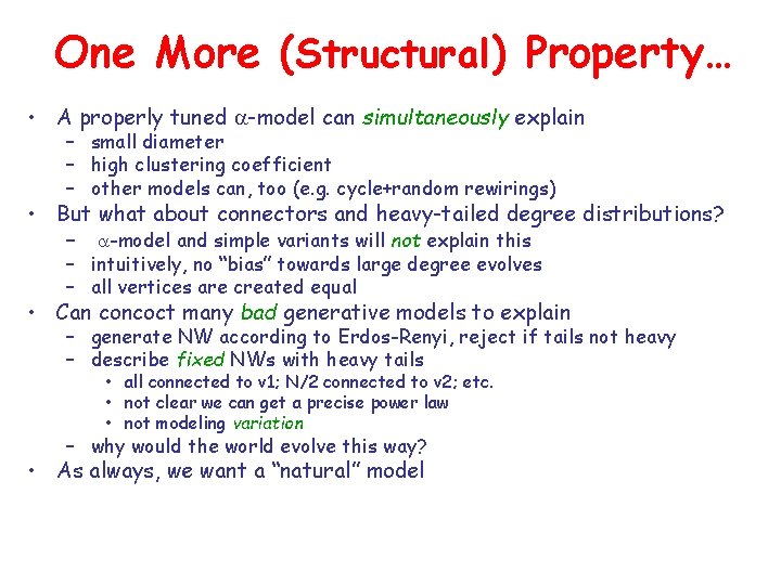
One More (Structural) Property… • A properly tuned a-model can simultaneously explain – small diameter – high clustering coefficient – other models can, too (e. g. cycle+random rewirings) • But what about connectors and heavy-tailed degree distributions? – a-model and simple variants will not explain this – intuitively, no “bias” towards large degree evolves – all vertices are created equal • Can concoct many bad generative models to explain – generate NW according to Erdos-Renyi, reject if tails not heavy – describe fixed NWs with heavy tails • all connected to v 1; N/2 connected to v 2; etc. • not clear we can get a precise power law • not modeling variation – why would the world evolve this way? • As always, we want a “natural” model

Quantifying Connectors: Heavy-Tailed Distributions

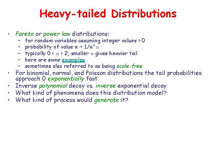
Heavy-tailed Distributions • Pareto or power law distributions: – – – for random variables assuming integer values > 0 probability of value x ~ 1/x^a typically 0 < a < 2; smaller a gives heavier tail here are some examples sometimes also referred to as being scale-free • For binomial, normal, and Poisson distributions the tail probabilities approach 0 exponentially fast • Inverse polynomial decay vs. inverse exponential decay • What kind of phenomena does this distribution model? • What kind of process would generate it?

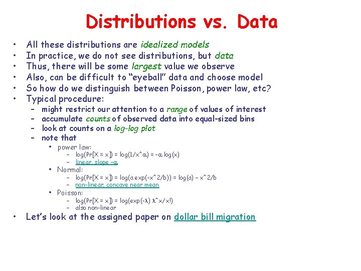
Distributions vs. Data • • • All these distributions are idealized models In practice, we do not see distributions, but data Thus, there will be some largest value we observe Also, can be difficult to “eyeball” data and choose model So how do we distinguish between Poisson, power law, etc? Typical procedure: – – might restrict our attention to a range of values of interest accumulate counts of observed data into equal-sized bins look at counts on a log-log plot note that • power law: – log(Pr[X = x]) = log(1/x^a) = -a log(x) – linear, slope –a • Normal: – log(Pr[X = x]) = log(a exp(-x^2/b)) = log(a) – x^2/b – non-linear, concave near mean • Poisson: • – log(Pr[X = x]) = log(exp(-l) l^x/x!) – also non-linear Let’s look at the assigned paper on dollar bill migration

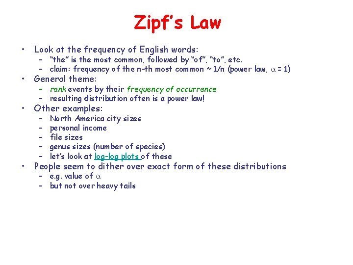
Zipf’s Law • Look at the frequency of English words: • General theme: • Other examples: • People seem to dither over exact form of these distributions – “the” is the most common, followed by “of”, “to”, etc. – claim: frequency of the n-th most common ~ 1/n (power law, a = 1) – rank events by their frequency of occurrence – resulting distribution often is a power law! – – – North America city sizes personal income file sizes genus sizes (number of species) let’s look at log-log plots of these – e. g. value of a – but not over heavy tails

Generating Heavy-Tailed Degrees: (Just) One Model

Preferential Attachment • Let’s warm up with a little Matlab demo… • • Start with (say) two vertices connected by an edge For i = 3 to N: – for each 1 <= j < i, let d(j) be degree of vertex j (so far) – let Z = S d(j) (sum of all degrees so far) – add new vertex i with k edges back to {1, …, i-1}: • i is connected back to j with probability d(j)/Z • might need to do some “smoothing” to deal with zero-degree vertices • • • Vertices j with high degree are likely to get more links! “Rich get richer” or “Matthew Effect” Natural model for many processes: • Generates a power law distribution of degrees • Let’s look at the Net. Logo simulation – hyperlinks on the web – new business and social contacts – transportation networks – exponent depends on value of k

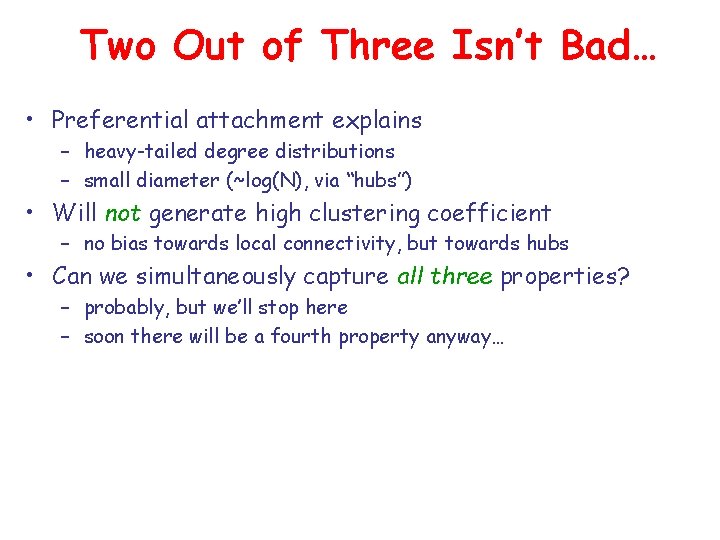
Two Out of Three Isn’t Bad… • Preferential attachment explains – heavy-tailed degree distributions – small diameter (~log(N), via “hubs”) • Will not generate high clustering coefficient – no bias towards local connectivity, but towards hubs • Can we simultaneously capture all three properties? – probably, but we’ll stop here – soon there will be a fourth property anyway…

Search and Navigation

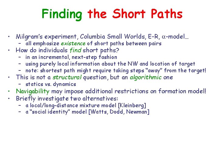
Finding the Short Paths • Milgram’s experiment, Columbia Small Worlds, E-R, a-model… – all emphasize existence of short paths between pairs • How do individuals find short paths? – in an incremental, next-step fashion – using purely local information about the NW and location of target – note: shortest path might require taking steps “away” from the target! • This is not a structural question, but an algorithmic one – statics vs. dynamics • Navigability may impose additional restrictions on formation model! • Briefly investigate two alternatives: – a local/long-distance mixture model [Kleinberg] – a “social identity” model [Watts, Dodd, Newman]

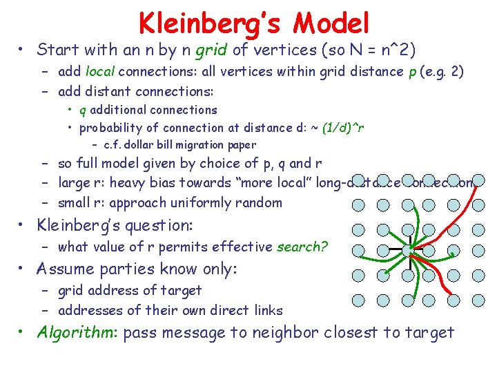
Kleinberg’s Model • Start with an n by n grid of vertices (so N = n^2) – add local connections: all vertices within grid distance p (e. g. 2) – add distant connections: • q additional connections • probability of connection at distance d: ~ (1/d)^r – c. f. dollar bill migration paper – so full model given by choice of p, q and r – large r: heavy bias towards “more local” long-distance connections – small r: approach uniformly random • Kleinberg’s question: – what value of r permits effective search? • Assume parties know only: – grid address of target – addresses of their own direct links • Algorithm: pass message to neighbor closest to target

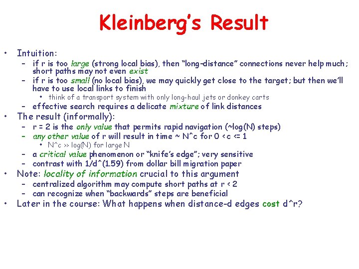
Kleinberg’s Result • Intuition: – if r is too large (strong local bias), then “long-distance” connections never help much; short paths may not even exist – if r is too small (no local bias), we may quickly get close to the target; but then we’ll have to use local links to finish • think of a transport system with only long-haul jets or donkey carts • – effective search requires a delicate mixture of link distances The result (informally): – r = 2 is the only value that permits rapid navigation (~log(N) steps) – any other value of r will result in time ~ N^c for 0 < c <= 1 • N^c >> log(N) for large N – a critical value phenomenon or “knife’s edge”; very sensitive – contrast with 1/d^(1. 59) from dollar bill migration paper • Note: locality of information crucial to this argument • Later in the course: What happens when distance-d edges cost d^r? – centralized algorithm may compute short paths at r < 2 – can recognize when “backwards” steps are beneficial

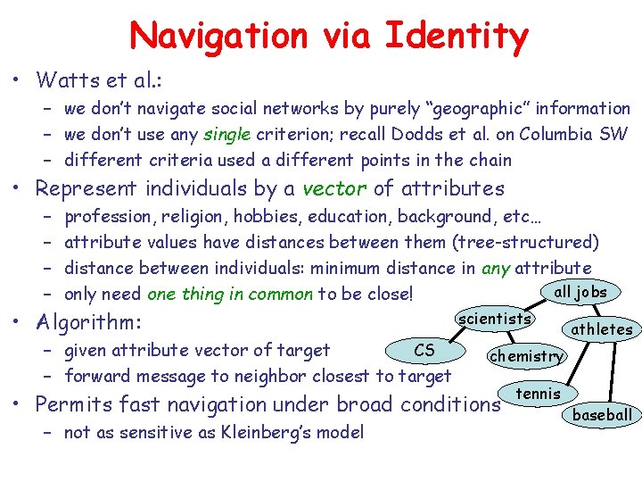
Navigation via Identity • Watts et al. : – we don’t navigate social networks by purely “geographic” information – we don’t use any single criterion; recall Dodds et al. on Columbia SW – different criteria used a different points in the chain • Represent individuals by a vector of attributes – – profession, religion, hobbies, education, background, etc… attribute values have distances between them (tree-structured) distance between individuals: minimum distance in any attribute all jobs only need one thing in common to be close! • Algorithm: – given attribute vector of target CS – forward message to neighbor closest to target scientists chemistry • Permits fast navigation under broad conditions – not as sensitive as Kleinberg’s model athletes tennis baseball