Inferring airsea fluxes through dynamically consistent ocean state

Inferring air-sea fluxes through dynamically consistent ocean state estimation Patrick Heimbach 1, 2 ICES/UTIG/JSG, The University of Texas at Austin, TX 2 EAPS, MIT, Cambridge, MA 1 Estimating the Circulation and Climate of the Ocean http: //ecco-group. org

Overview • Other reasons to care about Southern Ocean air-sea fluxes: – ice-to-sea fluxes – ice sheet-ocean interactions around Antarctica • Intercomparison of atmospheric reanalyses over the Southern Ocean & Antarctica • An inverse modeling and uncertainty quantification framework

Overview • Other reasons to care about Southern Ocean air-sea fluxes: – ice-to-sea fluxes – ice sheet-ocean interactions around Antarctica • Intercomparison of atmospheric reanalyses over the Southern Ocean & Antarctica • State estimation ≠ reanalysis • An inverse modeling and uncertainty quantification framework

Part 1: Ice sheet-ocean interactions around Antarctica

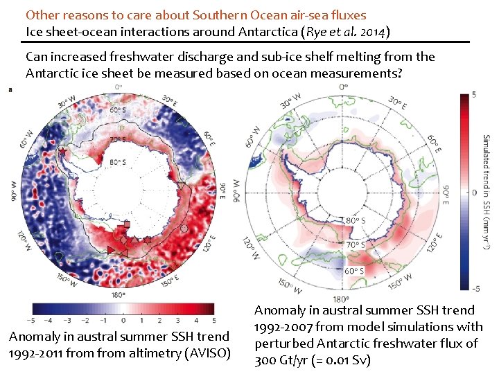
Other reasons to care about Southern Ocean air-sea fluxes Ice sheet-ocean interactions around Antarctica (Rye et al. 2014) Can increased freshwater discharge and sub-ice shelf melting from the Antarctic ice sheet be measured based on ocean measurements? Anomaly in austral summer SSH trend 1992 -2011 from altimetry (AVISO) Anomaly in austral summer SSH trend 1992 -2007 from model simulations with perturbed Antarctic freshwater flux of 300 Gt/yr (= 0. 01 Sv)

Part 2: Intercomparison of atmospheric reanalyses

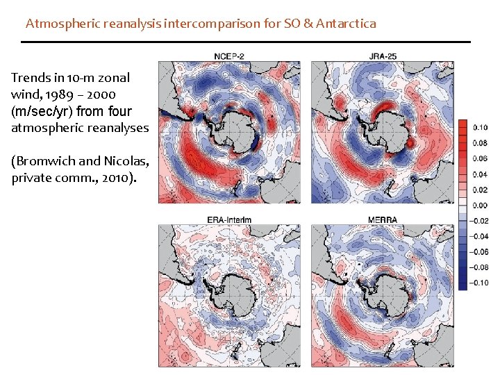
Atmospheric reanalysis intercomparison for SO & Antarctica Trends in 10 -m zonal wind, 1989 – 2000 (m/sec/yr) from four atmospheric reanalyses (Bromwich and Nicolas, private comm. , 2010).

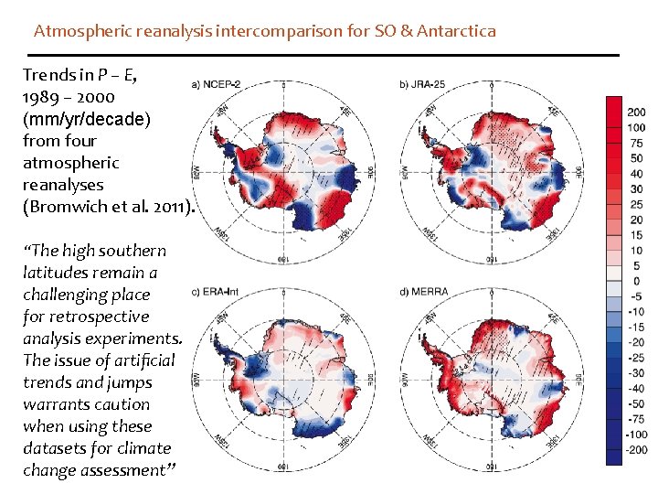
Atmospheric reanalysis intercomparison for SO & Antarctica Trends in P – E, 1989 – 2000 (mm/yr/decade) from four atmospheric reanalyses (Bromwich et al. 2011). “The high southern latitudes remain a challenging place for retrospective analysis experiments. The issue of artificial trends and jumps warrants caution when using these datasets for climate change assessment”

Part 3: State estimation (reconstruction) ≠ reanalysis (retrospective forecasting)

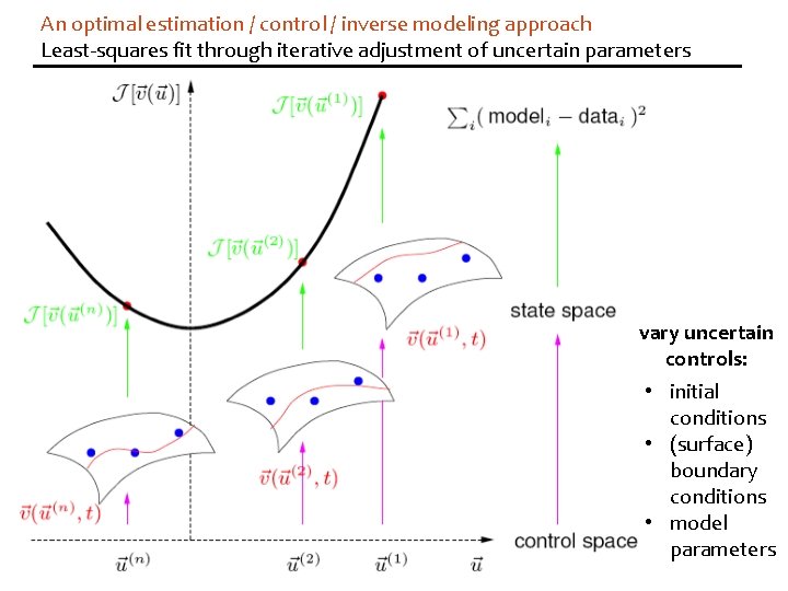
An optimal estimation / control / inverse modeling approach Least-squares fit through iterative adjustment of uncertain parameters vary uncertain controls: • initial conditions • (surface) boundary conditions • model parameters

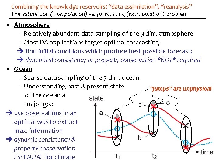
Combining the knowledge reservoirs: “data assimilation”, “reanalysis” The estimation (interpolation) vs. forecasting (extrapolation) problem • Atmosphere – Relatively abundant data sampling of the 3 -dim. atmosphere – Most DA applications target optimal forecasting find initial conditions which produce best possible forecast; dynamical consistency or property conservation *NOT* required • Ocean – Sparse data sampling of the 3 -dim. ocean – Understanding past & present state “jumps” are unphysical of the ocean a major goal use observations in an optimal way to extract max. information dynamic consistency & property conservation ESSENTIAL for climate

Balance the global (momentum, enthalpy, freshwater) budget !

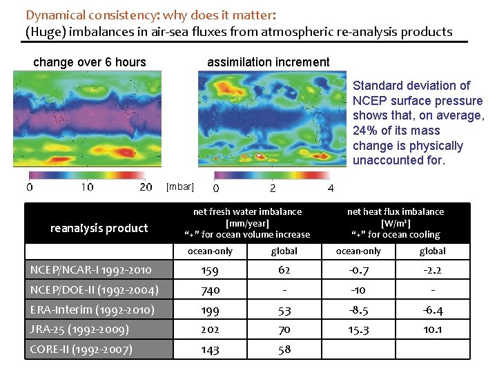
Dynamical consistency: why does it matter: (Huge) imbalances in air-sea fluxes from atmospheric re-analysis products change over 6 hours assimilation increment Standard deviation of NCEP surface pressure shows that, on average, 24% of its mass change is physically unaccounted for. [mbar] reanalysis product net fresh water imbalance [mm/year] “+” for ocean volume increase net heat flux imbalance [W/m 2] “+” for ocean cooling ocean-only global NCEP/NCAR-I 1992 -2010 159 62 -0. 7 -2. 2 NCEP/DOE-II (1992 -2004) 740 - -10 - ERA-Interim (1992 -2010) 199 53 -8. 5 -6. 4 JRA-25 (1992 -2009) 202 70 15. 3 10. 1 CORE-II (1992 -2007) 143 58

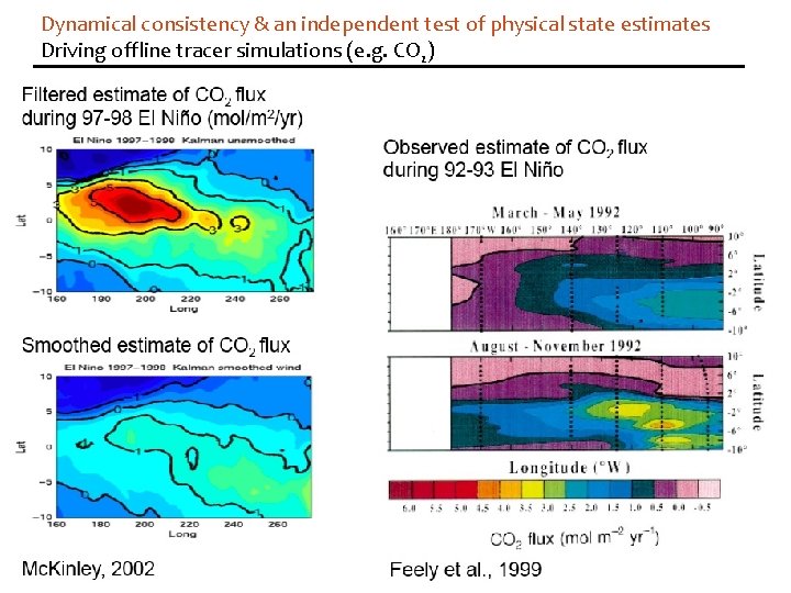
Dynamical consistency & an independent test of physical state estimates Driving offline tracer simulations (e. g. CO 2)

Part 4: An inverse modeling & uncertainty quantification framework

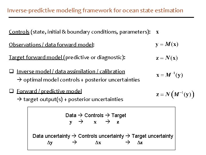
Inverse-predictive modeling framework for ocean state estimation Controls (state, initial & boundary conditions, parameters): Observations / data forward model: Target forward model (predictive or diagnostic): q Inverse model / data assimilation / calibration optimal model controls + posterior uncertainties q Forward / predictive model target output(s) + posterior uncertainties Data Controls Target y x z Data uncertainty Controls uncertainty Target uncertainty Δy Δx Δz

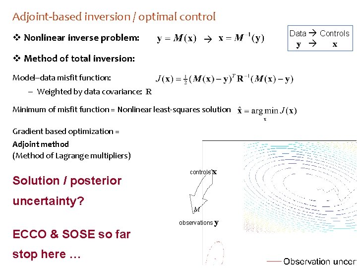
Adjoint-based inversion / optimal control v Nonlinear inverse problem: v Method of total inversion: Model–data misfit function: – Weighted by data covariance: R Minimum of misfit function = Nonlinear least-squares solution Gradient based optimization = Adjoint method (Method of Lagrange multipliers) Solution / posterior uncertainty? controls x M observations y ECCO & SOSE so far stop here … Data Controls y x

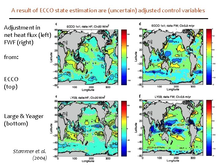
A result of ECCO state estimation are (uncertain) adjusted control variables Adjustment in net heat flux (left) FWF (right) from: ECCO (top) Large & Yeager (bottom) Stammer et al. (2004)

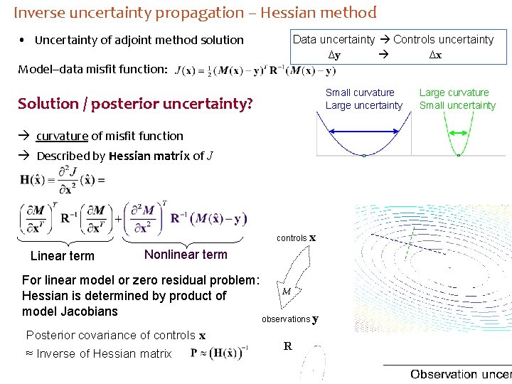
Inverse uncertainty propagation – Hessian method • Uncertainty of adjoint method solution Data uncertainty Controls uncertainty Δy Δx Model–data misfit function: Small curvature Large uncertainty Solution / posterior uncertainty? curvature of misfit function Described by Hessian matrix of J controls x Linear term Nonlinear term For linear model or zero residual problem: Hessian is determined by product of model Jacobians Posterior covariance of controls x ≈ Inverse of Hessian matrix M observations y R Large curvature Small uncertainty

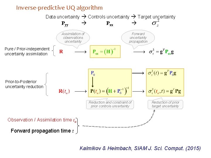
Inverse-predictive UQ algorithm Data uncertainty Controls uncertainty Target uncertainty Pyy Assimilation of observations uncertainty Pxx Forward uncertainty propagation Pure / Prior-independent uncertainty assimilation Prior-to-Posterior uncertainty reduction Reduction and constraint of prior controls uncertainty Reduction of prior target uncertainty Observation / Assimilation time ta Forward propagation time t Kalmikov & Heimbach, SIAM J. Sci. Comput. (2015)

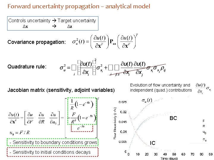
Forward uncertainty propagation – analytical model Controls uncertainty Target uncertainty Δx Δz Covariance propagation: Quadrature rule: Jacobian matrix (sensitivity, adjoint variables) Evolution of flow uncertainty and independent (quad. ) contributions BC - Sensitivity to boundary conditions grows - Sensitivity to initial conditions decays IC

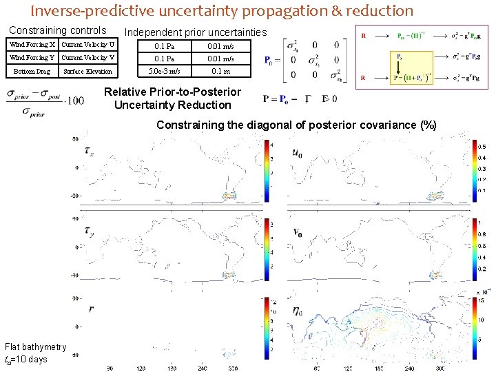
Inverse-predictive uncertainty propagation & reduction Constraining controls Independent prior uncertainties Wind Forcing X Current Velocity U 0. 1 Pa 0. 01 m/s Wind Forcing Y Current Velocity V 0. 1 Pa 0. 01 m/s 5. 0 e-3 m/s 0. 1 m Bottom Drag Surface Elevation Relative Prior-to-Posterior Uncertainty Reduction Constraining the diagonal of posterior covariance (%) Flat bathymetry ta=10 days

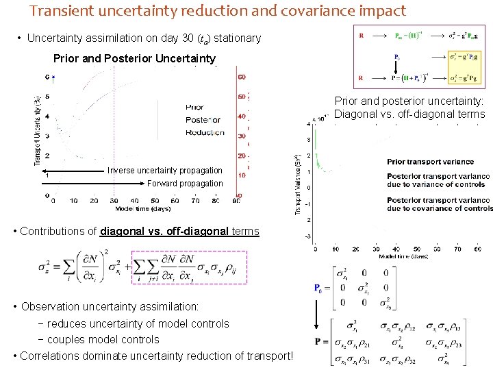
Transient uncertainty reduction and covariance impact • Uncertainty assimilation on day 30 (ta) stationary Prior and Posterior Uncertainty Prior and posterior uncertainty: Diagonal vs. off-diagonal terms Inverse uncertainty propagation Forward propagation • Contributions of diagonal vs. off-diagonal terms • Observation uncertainty assimilation: − reduces uncertainty of model controls − couples model controls • Correlations dominate uncertainty reduction of transport!

Some conclusions • Estimation / control method can be applied to invert for uncertain boundary fluxes from interior observations – surface fluxes constrained by hydrography (and altimetry) • Unlike most reanalyses, ECCO & SOSE state estimates place premium role on dynamical consistency – enable accurate partitioning of closed property budgets – posterior error covariance structure is carried by model dynamics i. e. , model propagators involved in Hessian matrix • State estimates so far do not quantify observation impact via Hessian – should be exploited more – computationally challenging