Game AI Path Finding 1 Introduction to Path

Game AI Path Finding 1

Introduction to Path Finding n n A Common Situation of Game AI Path Planning – From a start position to a destination point n Most Popular Technique – A* (A Star) » » 1968 A search algorithm Favorite teaching example : 15 -puzzle Algorithm that searches in a state space for the least costly path from start state to a goal state by examining the neighboring states 2

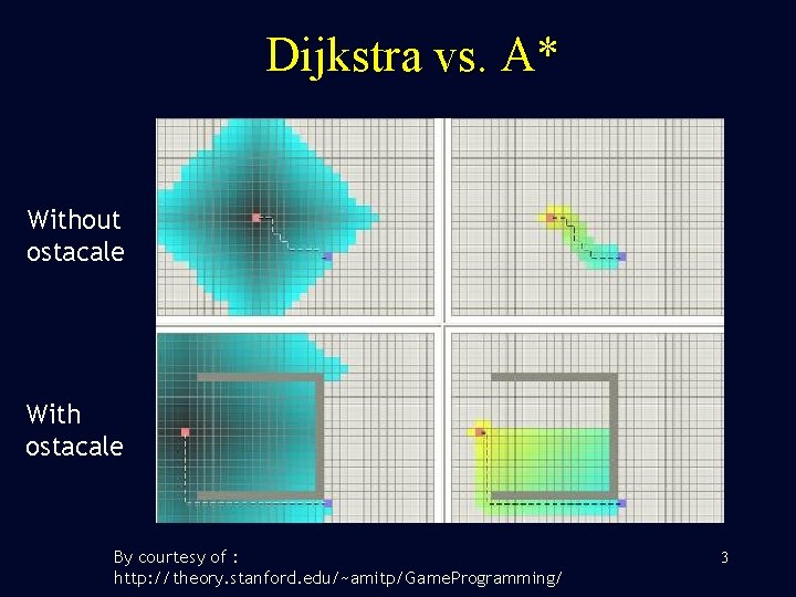
Dijkstra vs. A* Without ostacale With ostacale By courtesy of : http: //theory. stanford. edu/~amitp/Game. Programming/ 3

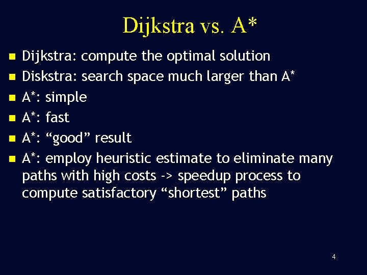
Dijkstra vs. A* n n n Dijkstra: compute the optimal solution Diskstra: search space much larger than A* A*: simple A*: fast A*: “good” result A*: employ heuristic estimate to eliminate many paths with high costs -> speedup process to compute satisfactory “shortest” paths 4

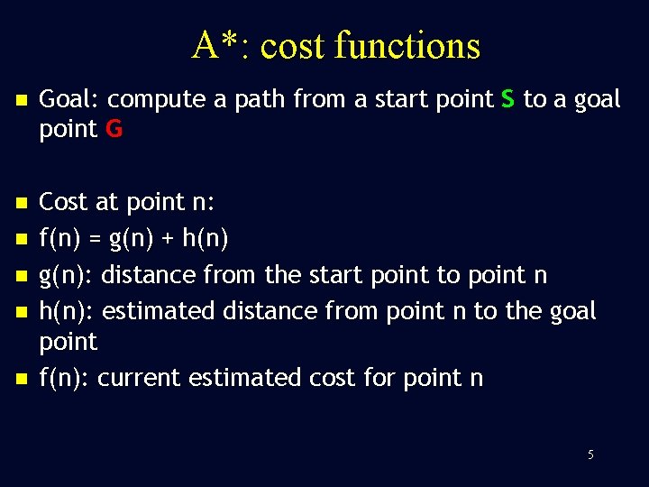
A*: cost functions n Goal: compute a path from a start point S to a goal point G n Cost at point n: f(n) = g(n) + h(n) g(n): distance from the start point to point n h(n): estimated distance from point n to the goal point f(n): current estimated cost for point n n n 5

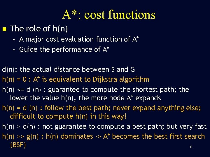
A*: cost functions n The role of h(n) – A major cost evaluation function of A* – Guide the performance of A* d(n): the actual distance between S and G h(n) = 0 : A* is equivalent to Dijkstra algorithm h(n) <= d (n) : guarantee to compute the shortest path; the lower the value h(n), the more node A* expands h(n) = d (n) : follow the best path; never expand anything else; difficult to compute h(n) in this way! h(n) > d(n) : not guarantee to compute a best path; but very fast h(n) >> g(n) : h(n) dominates -> A* becomes the best first search (BSF) 6

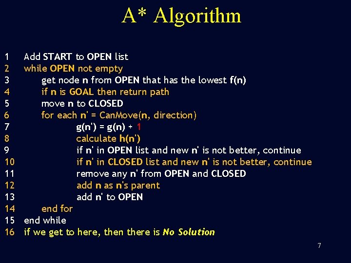
A* Algorithm 1 2 3 4 5 6 7 8 9 10 11 12 13 14 15 16 Add START to OPEN list while OPEN not empty get node n from OPEN that has the lowest f(n) if n is GOAL then return path move n to CLOSED for each n' = Can. Move(n, direction) g(n') = g(n) + 1 calculate h(n') if n' in OPEN list and new n' is not better, continue if n' in CLOSED list and new n' is not better, continue remove any n' from OPEN and CLOSED add n as n's parent add n' to OPEN end for end while if we get to here, then there is No Solution 7

A* Algorithm: Example -Show a grid map -Use Manhattan Distance to find the shortest path from the start point to the goal point 8

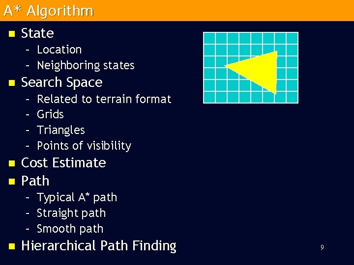
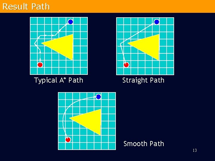
A* Algorithm n State – Location – Neighboring states n Search Space – – n n Related to terrain format Grids Triangles Points of visibility Cost Estimate Path – Typical A* path – Straight path – Smooth path n Hierarchical Path Finding 9

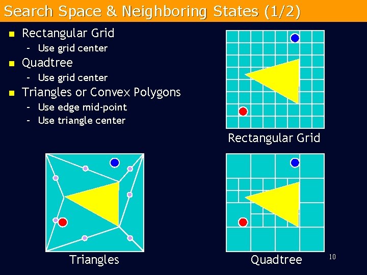
Search Space & Neighboring States (1/2) n Rectangular Grid – Use grid center n Quadtree – Use grid center n Triangles or Convex Polygons – Use edge mid-point – Use triangle center Rectangular Grid Triangles Quadtree 10

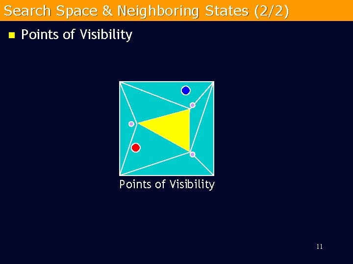
Search Space & Neighboring States (2/2) n Points of Visibility 11

Cost Estimate n Cost Function – g(n) – h(n) n Cost evaluation examples: – – – n Travel distance Travel time Fuel consumption Enemy and friendly regions … Estimate – Distance to goal 12

Result Path Typical A* Path Straight Path Smooth Path 13

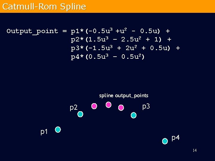
Catmull-Rom Spline Output_point = p 1*(-0. 5 u 3 +u 2 - 0. 5 u) + p 2*(1. 5 u 3 – 2. 5 u 2 + 1) + p 3*(-1. 5 u 3 + 2 u 2 + 0. 5 u) + p 4*(0. 5 u 3 – 0. 5 u 2) spline output_points p 2 p 1 p 3 p 4 14

Hierarchical Path Finding n Break the terrain into sub-regions – Room-to-room – 3 D layered terrain – Terrain LOD n Advantages: – Speedup the search – Solve the problem of layered path finding 15

Path Finding Challenges n Moving Goal – Do you need to find path each frame ? n Moving Obstacles – Prediction Scheme n Complexity of the terrain – Hierarchical path finding n “Good” path for Game AI, e. g. avoid enemies 16

References: http: //blog. minstrel. idv. tw/2004/12/star-algorithm. html http: //theory. stanford. edu/~amitp/Game. Programming/ 17