Excel Tips Tricks July 18 2019 2 Excel

Excel Tips & Tricks July 18, 2019

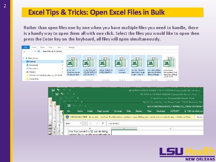
2 Excel Tips & Tricks: Open Excel Files in Bulk Rather than open files one by one when you have multiple files you need to handle, there is a handy way to open them all with one click. Select the files you would like to open then press the Enter key on the keyboard, all files will open simultaneously.

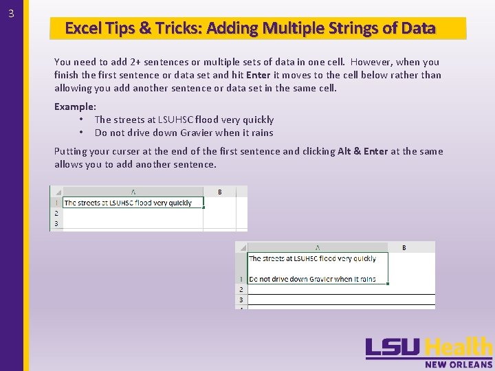
3 Excel Tips & Tricks: Adding Multiple Strings of Data You need to add 2+ sentences or multiple sets of data in one cell. However, when you finish the first sentence or data set and hit Enter it moves to the cell below rather than allowing you add another sentence or data set in the same cell. Example: • The streets at LSUHSC flood very quickly • Do not drive down Gravier when it rains Putting your curser at the end of the first sentence and clicking Alt & Enter at the same allows you to add another sentence.

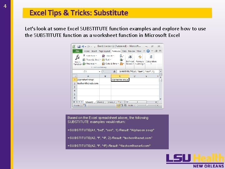
4 Excel Tips & Tricks: Substitute Let's look at some Excel SUBSTITUTE function examples and explore how to use the SUBSTITUTE function as a worksheet function in Microsoft Excel Based on the Excel spreadsheet above, the following SUBSTITUTE examples would return: =SUBSTITUTE(A 1, "bet", "con", 1) Result: "Alphacon soup" =SUBSTITUTE(A 2, "t", "4", 2) Result: "techon 4 henet. com“ =SUBSTITUTE(A 2, "t", "4") Result: "4 echon 4 hene 4. com"

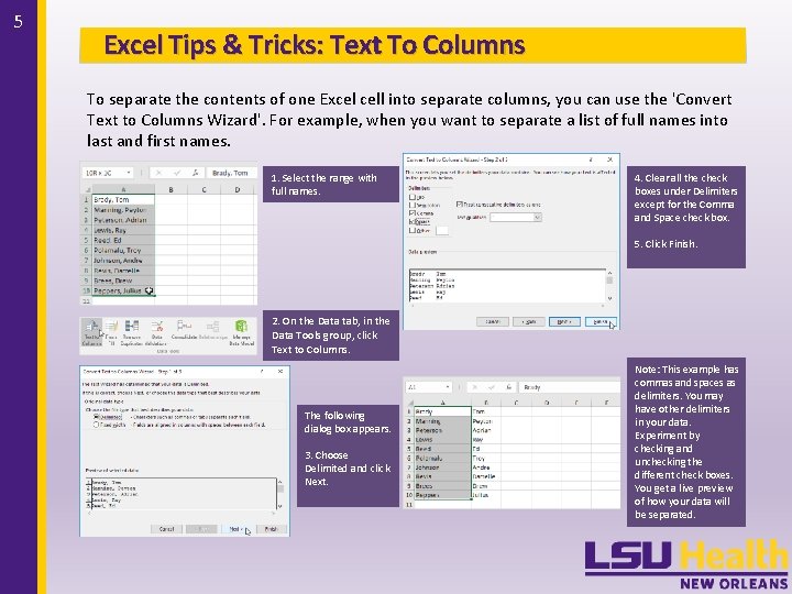
5 Excel Tips & Tricks: Text To Columns To separate the contents of one Excel cell into separate columns, you can use the 'Convert Text to Columns Wizard'. For example, when you want to separate a list of full names into last and first names. 1. Select the range with full names. 4. Clear all the check boxes under Delimiters except for the Comma and Space check box. 5. Click Finish. 2. On the Data tab, in the Data Tools group, click Text to Columns. The following dialog box appears. 3. Choose Delimited and click Next. Note: This example has commas and spaces as delimiters. You may have other delimiters in your data. Experiment by checking and unchecking the different check boxes. You get a live preview of how your data will be separated.

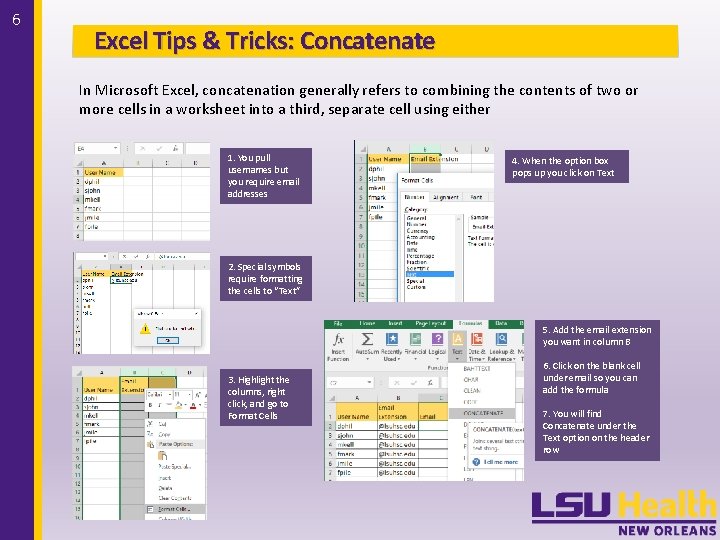
6 Excel Tips & Tricks: Concatenate In Microsoft Excel, concatenation generally refers to combining the contents of two or more cells in a worksheet into a third, separate cell using either 1. You pull usernames but you require email addresses 4. When the option box pops up you click on Text 2. Special symbols require formatting the cells to “Text” 5. Add the email extension you want in column B 3. Highlight the columns, right click, and go to Format Cells 6. Click on the blank cell under email so you can add the formula 7. You will find Concatenate under the Text option on the header row

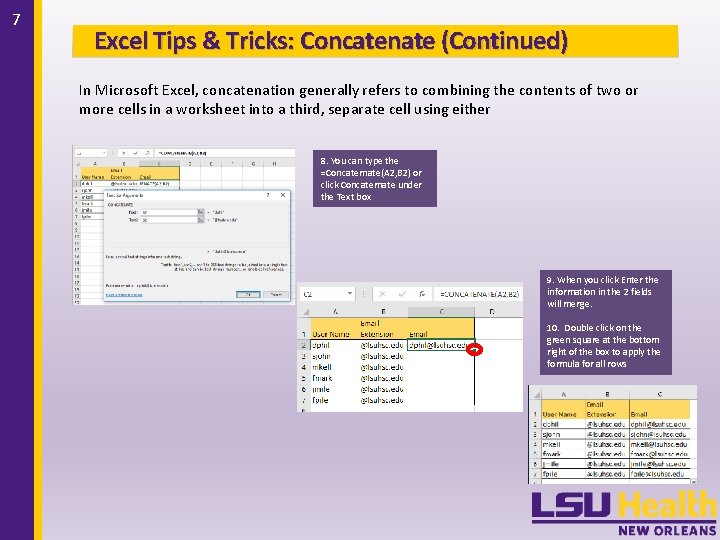
7 Excel Tips & Tricks: Concatenate (Continued) In Microsoft Excel, concatenation generally refers to combining the contents of two or more cells in a worksheet into a third, separate cell using either 8. You can type the =Concaternate(A 2, B 2) or click Concaternate under the Text box 9. When you click Enter the information in the 2 fields will merge. 10. Double click on the green square at the bottom right of the box to apply the formula for all rows

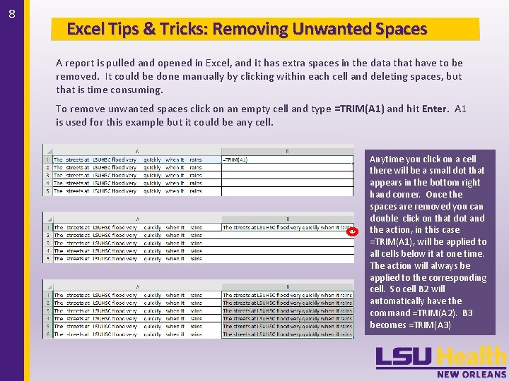
8 Excel Tips & Tricks: Removing Unwanted Spaces A report is pulled and opened in Excel, and it has extra spaces in the data that have to be removed. It could be done manually by clicking within each cell and deleting spaces, but that is time consuming. To remove unwanted spaces click on an empty cell and type =TRIM(A 1) and hit Enter. A 1 is used for this example but it could be any cell. Anytime you click on a cell there will be a small dot that appears in the bottom right hand corner. Once the spaces are removed you can double click on that dot and the action, in this case =TRIM(A 1), will be applied to all cells below it at one time. The action will always be applied to the corresponding cell. So cell B 2 will automatically have the command =TRIM(A 2). B 3 becomes =TRIM(A 3)

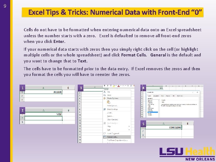
9 Excel Tips & Tricks: Numerical Data with Front-End “ 0” Cells do not have to be formatted when entering numerical data onto an Excel spreadsheet unless the number starts with a zero. Excel is defaulted to remove all front-end zeros when you click Enter. If your numerical data starts with zeros then you simply right click on the cell (or highlight multiple cells or the whole spreadsheet) and click Format Cells. General is the default and you want to change that to Text. The cells have to be formatted prior to the data entry. If Excel removes the zeros and then you format the cells you will have to reenter the zeros. 1 3 4 2 5

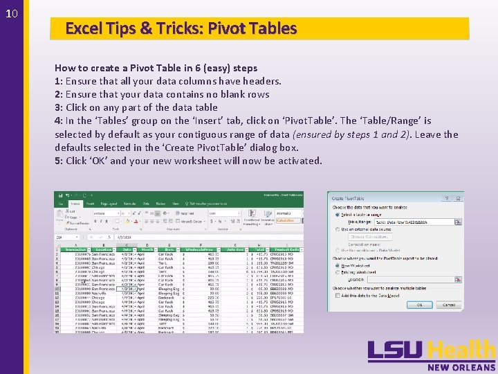
10 Excel Tips & Tricks: Pivot Tables How to create a Pivot Table in 6 (easy) steps 1: Ensure that all your data columns have headers. 2: Ensure that your data contains no blank rows 3: Click on any part of the data table 4: In the ‘Tables’ group on the ‘Insert’ tab, click on ‘Pivot. Table’. The ‘Table/Range’ is selected by default as your contiguous range of data (ensured by steps 1 and 2). Leave the defaults selected in the ‘Create Pivot. Table’ dialog box. 5: Click ‘OK’ and your new worksheet will now be activated.

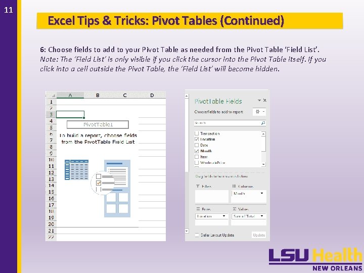
11 Excel Tips & Tricks: Pivot Tables (Continued) 6: Choose fields to add to your Pivot Table as needed from the Pivot Table ‘Field List’. Note: The ‘Field List’ is only visible if you click the cursor into the Pivot Table itself. If you click into a cell outside the Pivot Table, the ‘Field List’ will become hidden.

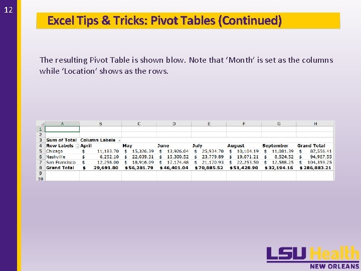
12 Excel Tips & Tricks: Pivot Tables (Continued) The resulting Pivot Table is shown blow. Note that ‘Month’ is set as the columns while ‘Location’ shows as the rows.