EE 381 K14 Multidimensional Digital Signal Processing Spring

EE 381 K-14 Multidimensional Digital Signal Processing Spring 2008 Introduction to Spectral Estimation Prof. Brian L. Evans Dept. of Electrical and Computer Engineering The University of Texas at Austin Lecture 13

Outline • Introduction • Nonparametric Methods • Parametric Methods • Conclusion 2

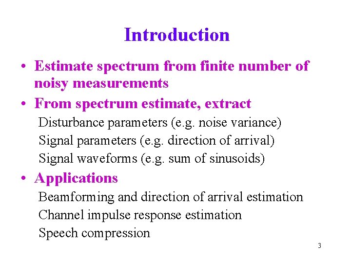
Introduction • Estimate spectrum from finite number of noisy measurements • From spectrum estimate, extract Disturbance parameters (e. g. noise variance) Signal parameters (e. g. direction of arrival) Signal waveforms (e. g. sum of sinusoids) • Applications Beamforming and direction of arrival estimation Channel impulse response estimation Speech compression 3

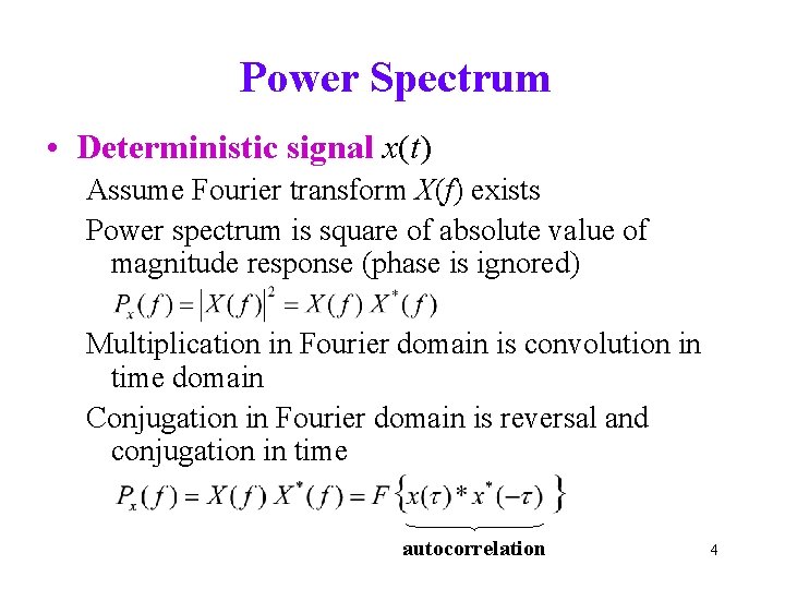
Power Spectrum • Deterministic signal x(t) Assume Fourier transform X(f) exists Power spectrum is square of absolute value of magnitude response (phase is ignored) Multiplication in Fourier domain is convolution in time domain Conjugation in Fourier domain is reversal and conjugation in time autocorrelation 4

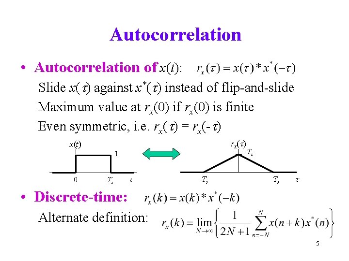
Autocorrelation • Autocorrelation of x(t): Slide x(t) against x*(t) instead of flip-and-slide Maximum value at rx(0) if rx(0) is finite Even symmetric, i. e. rx(t) = rx(-t) rx(t) 1 0 Ts t -Ts Ts Ts t • Discrete-time: Alternate definition: 5

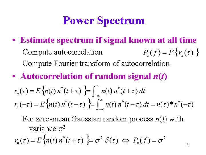
Power Spectrum • Estimate spectrum if signal known at all time Compute autocorrelation Compute Fourier transform of autocorrelation • Autocorrelation of random signal n(t) For zero-mean Gaussian random process n(t) with variance s 2 6

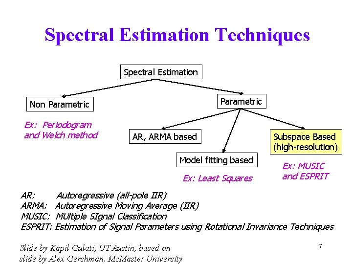
Spectral Estimation Techniques Spectral Estimation Parametric Non Parametric Ex: Periodogram and Welch method AR, ARMA based Model fitting based Ex: Least Squares Subspace Based (high-resolution) Ex: MUSIC and ESPRIT AR: Autoregressive (all-pole IIR) ARMA: Autoregressive Moving Average (IIR) MUSIC: MUltiple SIgnal Classification ESPRIT: Estimation of Signal Parameters using Rotational Invariance Techniques Slide by Kapil Gulati, UT Austin, based on slide by Alex Gershman, Mc. Master University 7

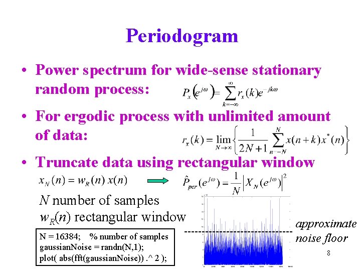
Periodogram • Power spectrum for wide-sense stationary random process: • For ergodic process with unlimited amount of data: • Truncate data using rectangular window N number of samples w. R(n) rectangular window N = 16384; % number of samples gaussian. Noise = randn(N, 1); plot( abs(fft(gaussian. Noise)). ^ 2 ); approximate noise floor 8

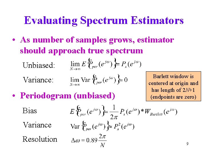
Evaluating Spectrum Estimators • As number of samples grows, estimator should approach true spectrum Unbiased: Variance: • Periodogram (unbiased) Barlett window is centered at origin and has length of 2 N+1 (endpoints are zero) Bias Variance Resolution 9

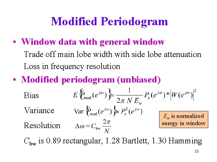
Modified Periodogram • Window data with general window Trade off main lobe width with side lobe attenuation Loss in frequency resolution • Modified periodogram (unbiased) Bias Variance Resolution Ew is normalized energy in window Cbw is 0. 89 rectangular, 1. 28 Bartlett, 1. 30 Hamming 10

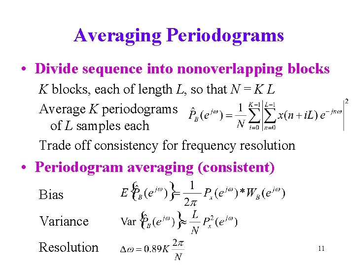
Averaging Periodograms • Divide sequence into nonoverlapping blocks K blocks, each of length L, so that N = K L Average K periodograms of L samples each Trade off consistency for frequency resolution • Periodogram averaging (consistent) Bias Variance Resolution 11

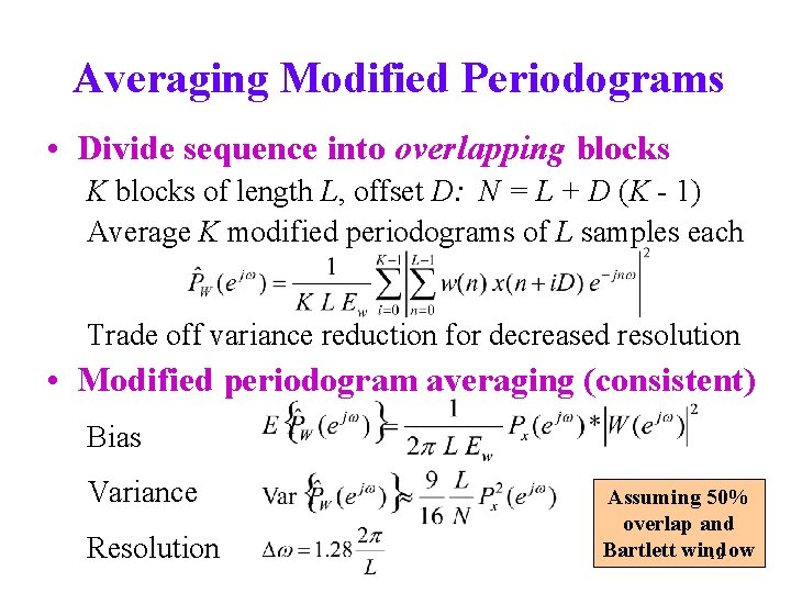
Averaging Modified Periodograms • Divide sequence into overlapping blocks K blocks of length L, offset D: N = L + D (K - 1) Average K modified periodograms of L samples each Trade off variance reduction for decreased resolution • Modified periodogram averaging (consistent) Bias Variance Resolution Assuming 50% overlap and Bartlett window 12

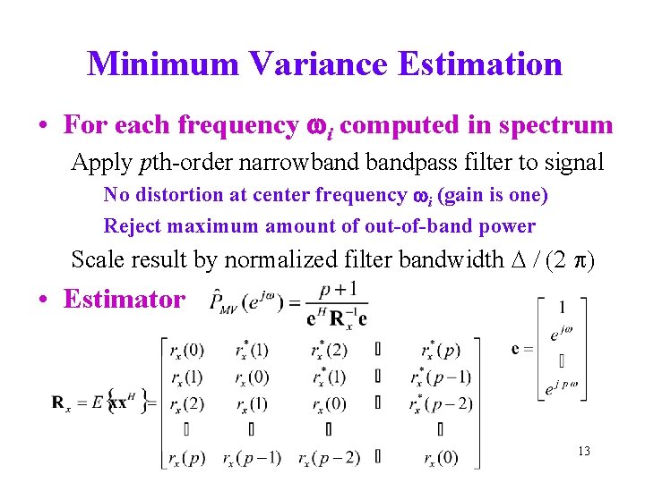
Minimum Variance Estimation • For each frequency wi computed in spectrum Apply pth-order narrowbandpass filter to signal No distortion at center frequency wi (gain is one) Reject maximum amount of out-of-band power Scale result by normalized filter bandwidth D / (2 p) • Estimator 13

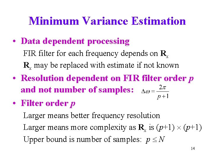
Minimum Variance Estimation • Data dependent processing FIR filter for each frequency depends on Rx Rx may be replaced with estimate if not known • Resolution dependent on FIR filter order p and not number of samples: • Filter order p Larger means better frequency resolution Larger means more complexity as Rx is (p+1) Upper bound is number of samples: p N 14