Economics and Law Lecture 3 Ross Anderson Demand

Economics and Law Lecture 3 Ross Anderson

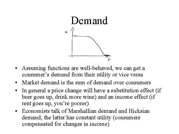
Demand • Assuming functions are well-behaved, we can get a consumer’s demand from their utility or vice versa • Market demand is the sum of demand over consumers • In general a price change will have a substitution effect (if beer goes up, drink more wine) and an income effect (if rent goes up, you’re poorer) • Economists talk of Marshallian demand Hicksian demand; the latter has constant utility (consumers compensated for changes in income)

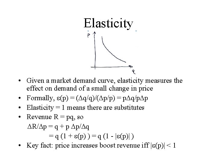
Elasticity • Given a market demand curve, elasticity measures the effect on demand of a small change in price • Formally, (p) = ( q/q)/( p/p) = p q/p p • Elasticity = 1 means there are substitutes • Revenue R = pq, so R/ p = q + p p/ q = q (1 + (p) ) = q (1 - | (p)| ) • Key fact: price increases boost revenue iff | (p)| < 1

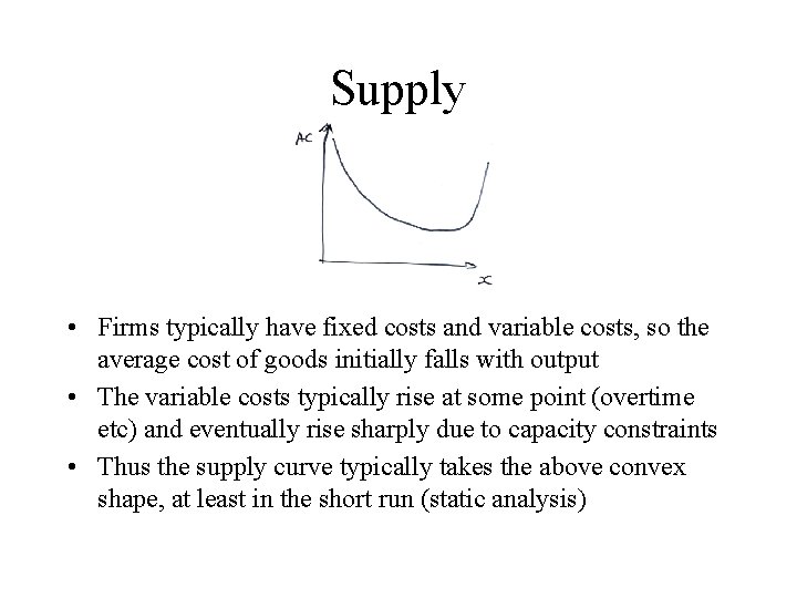
Supply • Firms typically have fixed costs and variable costs, so the average cost of goods initially falls with output • The variable costs typically rise at some point (overtime etc) and eventually rise sharply due to capacity constraints • Thus the supply curve typically takes the above convex shape, at least in the short run (static analysis)

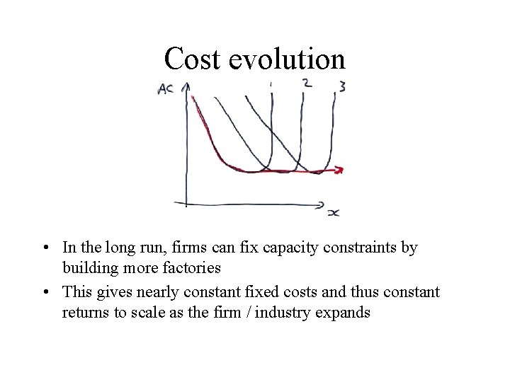
Cost evolution • In the long run, firms can fix capacity constraints by building more factories • This gives nearly constant fixed costs and thus constant returns to scale as the firm / industry expands

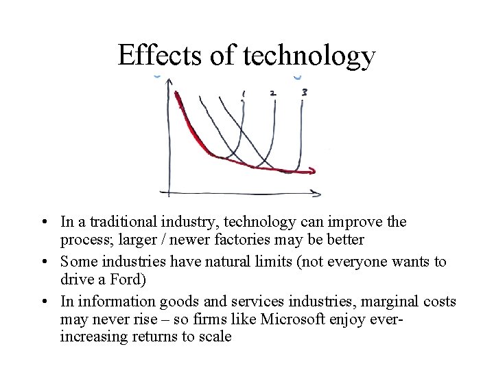
Effects of technology • In a traditional industry, technology can improve the process; larger / newer factories may be better • Some industries have natural limits (not everyone wants to drive a Ford) • In information goods and services industries, marginal costs may never rise – so firms like Microsoft enjoy everincreasing returns to scale

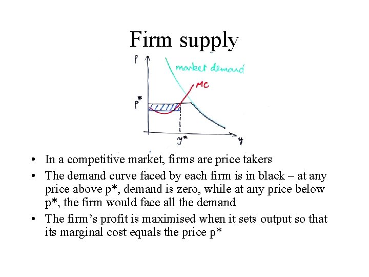
Firm supply • In a competitive market, firms are price takers • The demand curve faced by each firm is in black – at any price above p*, demand is zero, while at any price below p*, the firm would face all the demand • The firm’s profit is maximised when it sets output so that its marginal cost equals the price p*

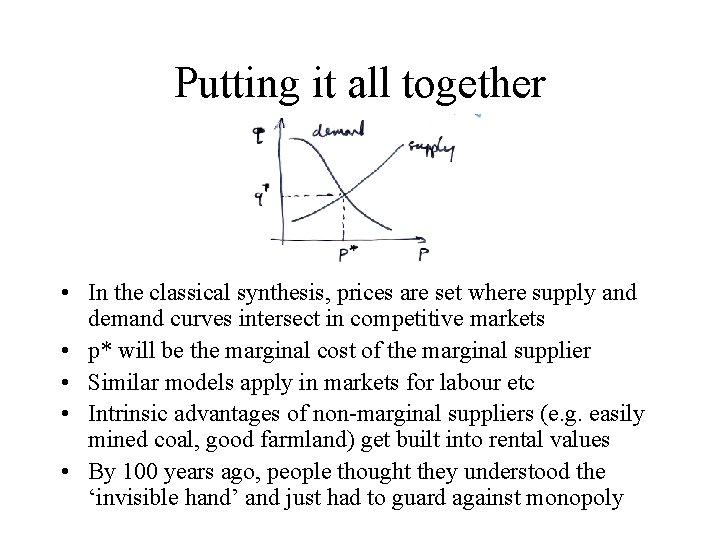
Putting it all together • In the classical synthesis, prices are set where supply and demand curves intersect in competitive markets • p* will be the marginal cost of the marginal supplier • Similar models apply in markets for labour etc • Intrinsic advantages of non-marginal suppliers (e. g. easily mined coal, good farmland) get built into rental values • By 100 years ago, people thought they understood the ‘invisible hand’ and just had to guard against monopoly

Equilibrium • Studying supply and demand for one good is ‘partial equilibrium analysis’. ‘General equilibrium analysis’ adds in labour, capital etc • First theorem of welfare economics: market equilibrium is Pareto optimal • Second theorem: any Pareto optimal allocation can be achieved by market forces promided preferences are convex • Technical conditions include rational actors, property rights, complete information, no transaction costs … (more later)

Efficiency, welfare and justice • These are different concepts! Giving the king all the money is Pareto efficient • Different theories of justice are consistent with different welfare functions – W = ∑Ui is classicial utilitarian welfare – W = min Ui is Rawlsian welfare – that of the most miserable citizen • Pigou: diminishing marginal utility of money means that transferring £ 1 from a rich man to a poor one will generally increase welfare • But – there’s a methodological problem!

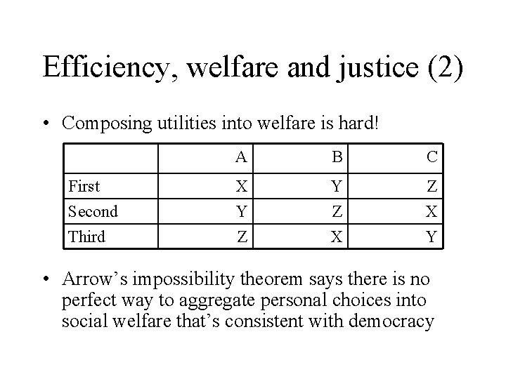
Efficiency, welfare and justice (2) • Composing utilities into welfare is hard! First Second Third A B C X Y Z X Z X Y • Arrow’s impossibility theorem says there is no perfect way to aggregate personal choices into social welfare that’s consistent with democracy

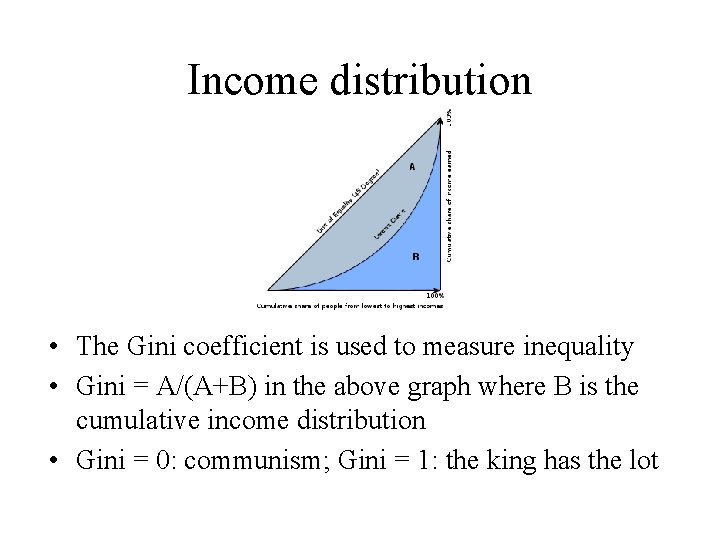
Income distribution • The Gini coefficient is used to measure inequality • Gini = A/(A+B) in the above graph where B is the cumulative income distribution • Gini = 0: communism; Gini = 1: the king has the lot

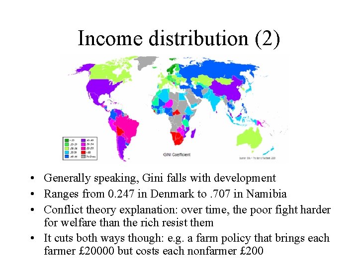
Income distribution (2) • Generally speaking, Gini falls with development • Ranges from 0. 247 in Denmark to. 707 in Namibia • Conflict theory explanation: over time, the poor fight harder for welfare than the rich resist them • It cuts both ways though: e. g. a farm policy that brings each farmer £ 20000 but costs each nonfarmer £ 200

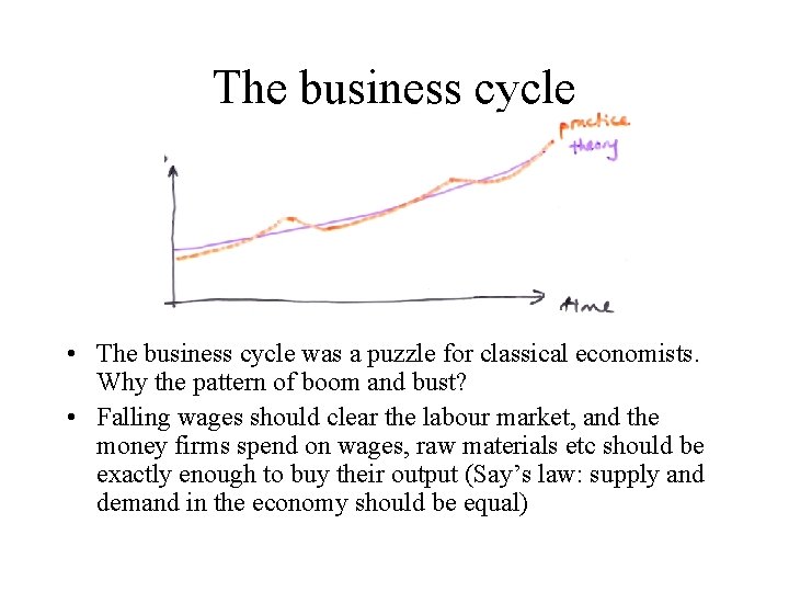
The business cycle • The business cycle was a puzzle for classical economists. Why the pattern of boom and bust? • Falling wages should clear the labour market, and the money firms spend on wages, raw materials etc should be exactly enough to buy their output (Say’s law: supply and demand in the economy should be equal)

The business cycle (2) • Mill and Ricardo argued that demand for goods + savings = supply of goods + investment, and savings = investment, so demand = supply • Malthus and Sismondi argued that savings and investment could differ in the short term; falling confidence people hoard cash • 1930 s: Keynes elaborated this with ‘liquidity preference’. People want a certain level of savings – maybe 3 months’ salary. In a recession, liquidity preference rises • Many other dynamic effects, different timescales…

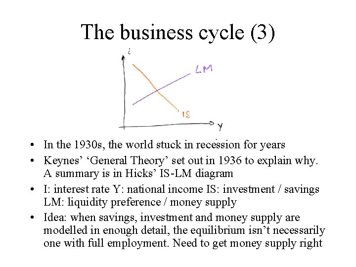
The business cycle (3) • In the 1930 s, the world stuck in recession for years • Keynes’ ‘General Theory’ set out in 1936 to explain why. A summary is in Hicks’ IS-LM diagram • I: interest rate Y: national income IS: investment / savings LM: liquidity preference / money supply • Idea: when savings, investment and money supply are modelled in enough detail, the equilibrium isn’t necessarily one with full employment. Need to get money supply right

The business cycle (4) • Credit introduces instability at many levels. • In a boom, people and firms borrow assets that appreciate faster than the interest costs • A bank that takes in £ 100 in deposits might lend out £ 94; so £ 6 of capital underwrites £ 94 of lending – a multiplier of 94/6 = 15. 7 • In a recession many things happen at once: – – Some loans go bad, eating into capital The bank’s share price falls, further eating capital The regulator raises capital requirements from 6% to 8% The government competes for the available loans • So the money supply contracts sharply

The current recession • Kicked off by US subprime mortgage crisis of 2007 which led to collapse of money markets – no bank knew which other banks were still sound • A common pattern – see Reinhart & Rogoff • Big question: will the recession be – Small (2 y, asset price fall 30%) – Medium (4 y, asset price fall 50%) – Large (8 y, asset price fall 80%) • History tells of two biggies (US 1930 s, Japan 1990 s); dozens of medium; very many small • UK: questions over budget deficit, house prices

Recession and tech • Recessions may be fed by bubbles and triggered by financial markets but are often tried up with tech change • Railways 1840 s, cars 1920 s, tech 1990 s – boom creates capacity, bust drives down prices • Schumpeter: ‘creative destruction’ • Tech doing much better now than 2001 -2: some suffer (Sun, Motorola) but most firms thriving • Jan 2010 Microsoft profits up 60%, Google 17%… • IT now a thoroughly global industry: if the USA does better than Europe, or people buy consumer electronics instead of cars, we still get our share

Recession and tech (2) • Known patterns: capital goods hit first in recession (e. g. new car sales down 30 -50%) • Services fairly stable thanks to many long-term facilities management contracts • Outsourcing booming as firms cut costs • Financial sector IT is struggling (like 1991) • Government systems folks confident (though Conservatives say they’ll cut waste) • Hardware is always cyclical – fab capex down a bit but firms know they must keep investing • When will Moore’s law run out?