Econometric Causality James Heckman 2008 International Statistical Review

Econometric Causality James Heckman (2008). International Statistical Review

James Heckman • Nobel prize in economics (2000) • Developed the “two-stage method” to allow researchers to correct for selection bias

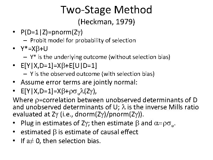
Two-Stage Method (Heckman, 1979) • P(D=1|Z)=pnorm(Zg) – Probit model for probability of selection • Y*=Xb+U – Y* is the underlying outcome (without selection bias) • E[Y|X, D=1]=Xb+E[U|D=1] – Y is the observed outcome (with selection bias) • Assume error terms are jointly normal: • E[Y|X, D=1]=Xb+rsul(Zg), Where r=correlation between unobserved determinants of D and unobserved determinants of U; l is the inverse Mills ratio evaluated at Zg (i. e. , dnorm(Zg)/pnorm(Zg)). • Plug in estimates of Zg; then estimate b and a=rsu. • estimated b is estimate of causal effect • If a≠ 0, then selection bias.

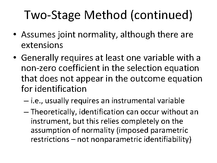
Two-Stage Method (continued) • Assumes joint normality, although there are extensions • Generally requires at least one variable with a non-zero coefficient in the selection equation that does not appear in the outcome equation for identification – i. e. , usually requires an instrumental variable – Theoretically, identification can occur without an instrument, but this relies completely on the assumption of normality (imposed parametric restrictions – not nonparametric identifiability)

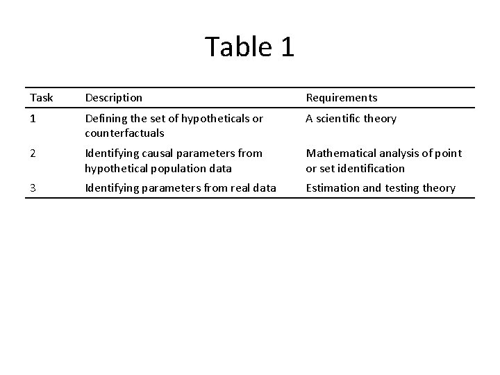
Table 1 Task Description Requirements 1 Defining the set of hypotheticals or counterfactuals A scientific theory 2 Identifying causal parameters from hypothetical population data Mathematical analysis of point or set identification 3 Identifying parameters from real data Estimation and testing theory

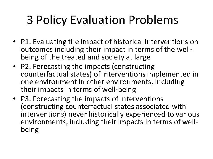
3 Policy Evaluation Problems • P 1. Evaluating the impact of historical interventions on outcomes including their impact in terms of the wellbeing of the treated and society at large • P 2. Forecasting the impacts (constructing counterfactual states) of interventions implemented in one environment in other environments, including their impacts in terms of well-being • P 3. Forecasting the impacts of interventions (constructing counterfactual states associated with interventions) never historically experienced to various environments, including their impacts in terms of wellbeing

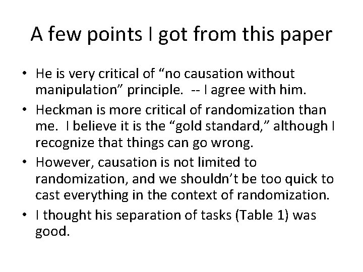
A few points I got from this paper • He is very critical of “no causation without manipulation” principle. -- I agree with him. • Heckman is more critical of randomization than me. I believe it is the “gold standard, ” although I recognize that things can go wrong. • However, causation is not limited to randomization, and we shouldn’t be too quick to cast everything in the context of randomization. • I thought his separation of tasks (Table 1) was good.

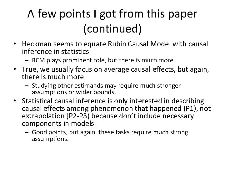
A few points I got from this paper (continued) • Heckman seems to equate Rubin Causal Model with causal inference in statistics. – RCM plays prominent role, but there is much more. • True, we usually focus on average causal effects, but again, there is much more. – Studying other estimands may require much stronger assumptions or wider bounds. • Statistical causal inference is only interested in describing causal effects among phenomenon that happened (P 1), not extrapolation (P 2 -P 3) because don’t include necessary components in models. – Good points, but again, these tasks require much strong assumptions.

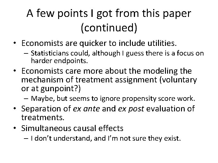
A few points I got from this paper (continued) • Economists are quicker to include utilities. – Statisticians could, although I guess there is a focus on harder endpoints. • Economists care more about the modeling the mechanism of treatment assignment (voluntary or at gunpoint? ) – Maybe, but seems to ignore propensity score work. • Separation of ex ante and ex post evaluation of treatments. • Simultaneous causal effects – I don’t understand, and I’m not sure they exist.

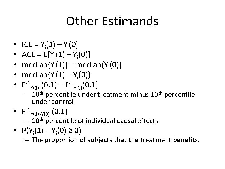
Other Estimands • • • ICE = Yi(1) – Yi(0) ACE = E[Yi(1) – Yi(0)] median{Yi(1)} – median{Yi(0)} median{Yi(1) – Yi(0)} F-1 Y(1) (0. 1) – F-1 Y(0)(0. 1) – 10 th percentile under treatment minus 10 th percentile under control • F-1 Y(1)-Y(0) (0. 1) – 10 th percentile of individual causal effects • P(Yi(1) – Yi(0) ≥ 0) – The proportion of subjects that the treatment benefits.

Bounds for P[Yi(1) ≥ Yi(0)] • RCT identifies F 1(y)=P(Yi(1) ≤ y) and F 0(x)=P(Yi(0) ≤ x) • Need to identify joint distribution: H(x, y)=P(Yi(0) ≤ x, Yi(1) ≤ x) • Without additional assumptions, best one can do is come up with bounds. • max{F 0(x)+F 1(y)-1, 0} ≤ H(x, y) ≤ min{F 0(x), F 1(y)} – Frechet-Hoeffding Bounds – Denote bounds as W(x, y) and M(x, y) • P[Yi(1) ≥ Yi(0)] = ∫y∫y>x. H(x, y)dxdy • ∫y∫y>x. W(x, y)dxdy ≤ P[Yi(1) ≥ Yi(0)] ≤ ∫y∫y>x. M(x, y)dxdys.