Ecology 8310 Population and Community Ecology Deterministic vs

Ecology 8310 Population (and Community) Ecology • Deterministic vs. stochastic models • Sources of variation • Environmental stochasticity in discrete (and continuous) time models • Demographic stochasticity • Melbourne and Hastings (2008)

Deterministic models: • Exactly predict the future state of the system (given starting conditions and parameter values). • If repeated, with same conditions, the outcome will be identical. • This is useful (and easier to analyze), but unrealistic. • Hence, we might use stochastic models…

Stochastic models: Variation can have effects on: • population size • variation in population size • Extinction risk

Sources of variation: Demographic stochasticity • Classically: random variation in N arising because of the probabilistic nature of births and deaths. Extinction caused by low N and "unfortunate coincidences" (Melbourne and Hastings 2008) in fate of individuals. High N smooths out this variation. • Stochastic sex determination = random variation in the production females vs. males. • Demographic heterogeneity = variation (random or deterministic) among individuals in vital rates.

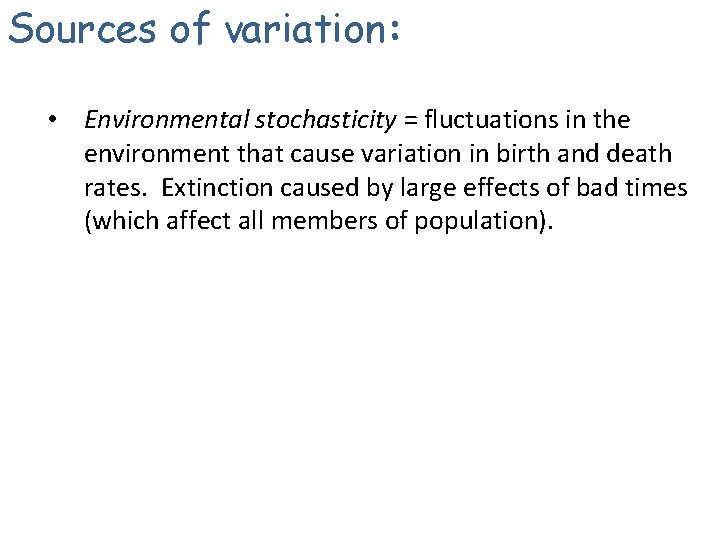
Sources of variation: • Environmental stochasticity = fluctuations in the environment that cause variation in birth and death rates. Extinction caused by large effects of bad times (which affect all members of population).

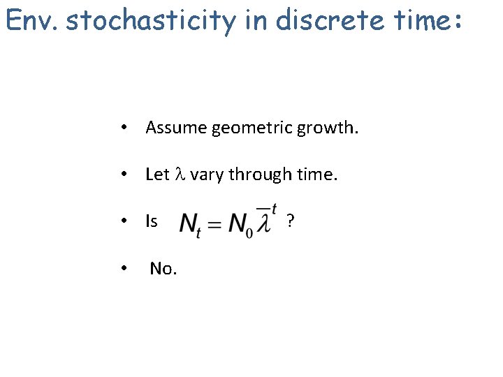
Env. stochasticity in discrete time: • Assume geometric growth. • Let l vary through time. • Is • No. ?

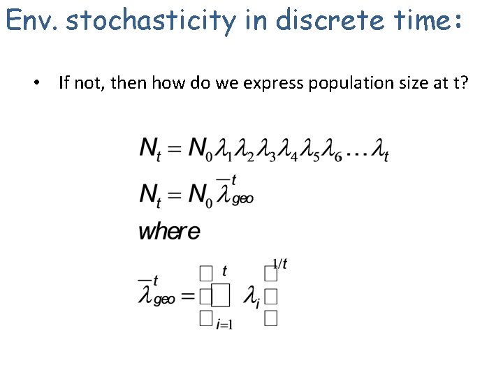
Env. stochasticity in discrete time: • If not, then how do we express population size at t?

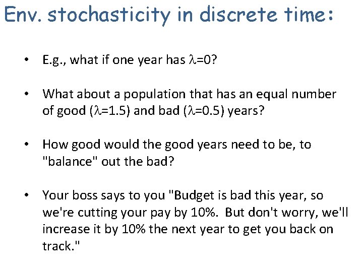
Env. stochasticity in discrete time: • E. g. , what if one year has l=0? • What about a population that has an equal number of good (l=1. 5) and bad (l=0. 5) years? • How good would the good years need to be, to "balance" out the bad? • Your boss says to you "Budget is bad this year, so we're cutting your pay by 10%. But don't worry, we'll increase it by 10% the next year to get you back on track. "

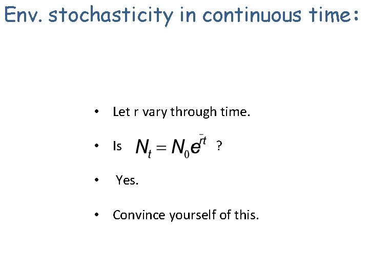
Env. stochasticity in continuous time: • Let r vary through time. • Is • ? Yes. • Convince yourself of this.

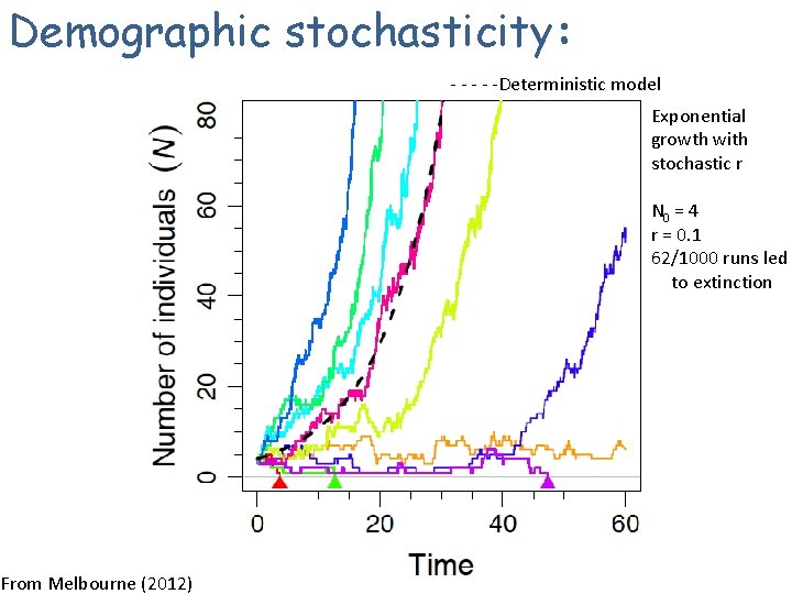
Demographic stochasticity: • What about demographic stochasticity? • Recall that in its pure form, all individuals have the same death and birth rates. • But, because births and deaths are discrete and probabilistic, demographic stochasticity arises… • And is most important at small N. • Easiest to illustrate with simulations.

Demographic stochasticity: - - -Deterministic model Exponential growth with stochastic r N 0 = 4 r = 0. 1 62/1000 runs led to extinction From Melbourne (2012)

Demographic heterogeneity: • But individuals are not identical (different size, local resource conditions, nutritional state, etc. ). • This introduces variation in demographic rates. • E. g. , imagine individuals vary in their mortality rate? Draw a survivorship curve for populations with the same mean survival, but different variances…

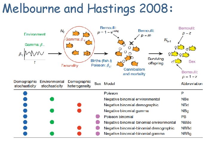
Melbourne and Hastings 2008: • Ricker model: E[Nt+1] = RNte-a. Nt • Incorporated variation due to: • Environment • Sex ratio • Birth and death • Demographic heterogeneity • Simulated and examined effect on time to extinction

Melbourne and Hastings 2008: • Ricker model: E[Nt+1] = RNte-a. Nt • Incorporated variation due to: • Environment • Sex ratio • Birth and death • Demographic heterogeneity • Simulated and examined effect on time to extinction

Melbourne and Hastings 2008:

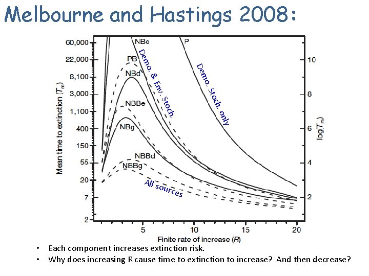
Melbourne and Hastings 2008: o. & Dem o. S nly h. o . och . St toc Env All s ourc es • Each component increases extinction risk. • Why does increasing R cause time to extinction to increase? And then decrease?

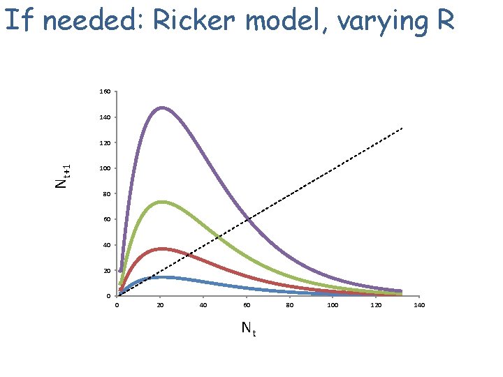
If needed: Ricker model, varying R 160 140 Nt+1 120 100 80 60 40 20 0 0 20 40 60 Nt 80 100 120 140

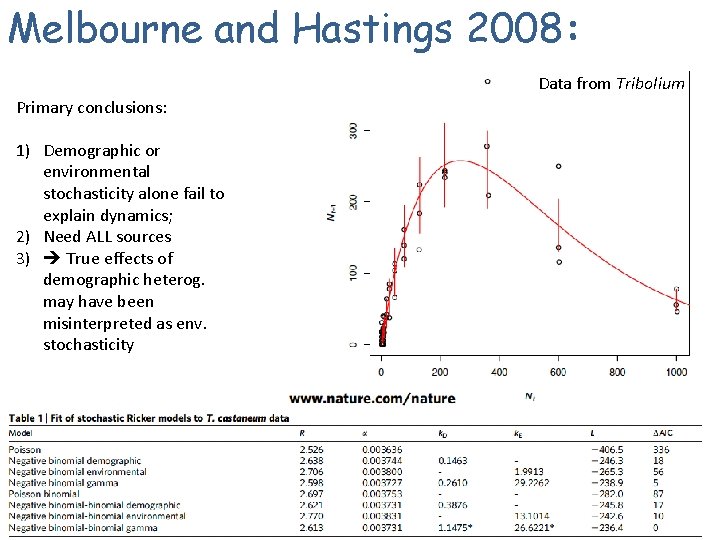
Melbourne and Hastings 2008: Data from Tribolium Primary conclusions: 1) Demographic or environmental stochasticity alone fail to explain dynamics; 2) Need ALL sources 3) True effects of demographic heterog. may have been misinterpreted as env. stochasticity

Discussion: Spatial and Demographic Heterogeneity: • Imagine two patches with different growth rates. What is the long-term growth of the aggregate system? • Imagine two types of individuals ("slow" and "fast"). What is the long-term growth of the population?