ECE 8443 Pattern Recognition LECTURE 08 DIMENSIONALITY PRINCIPAL

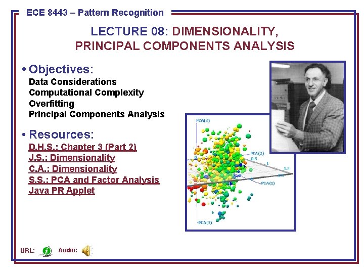
ECE 8443 – Pattern Recognition LECTURE 08: DIMENSIONALITY, PRINCIPAL COMPONENTS ANALYSIS • Objectives: Data Considerations Computational Complexity Overfitting Principal Components Analysis • Resources: D. H. S. : Chapter 3 (Part 2) J. S. : Dimensionality C. A. : Dimensionality S. S. : PCA and Factor Analysis Java PR Applet URL: Audio:

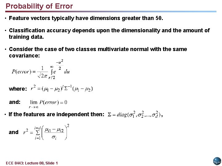
Probability of Error • Feature vectors typically have dimensions greater than 50. • Classification accuracy depends upon the dimensionality and the amount of training data. • Consider the case of two classes multivariate normal with the same covariance: where: and: • If the features are independent then: and ECE 8443: Lecture 08, Slide 1 ,

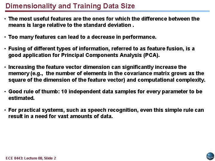
Dimensionality and Training Data Size • The most useful features are the ones for which the difference between the means is large relative to the standard deviation. • Too many features can lead to a decrease in performance. • Fusing of different types of information, referred to as feature fusion, is a good application for Principal Components Analysis (PCA). • Increasing the feature vector dimension can significantly increase the memory (e. g. , the number of elements in the covariance matrix grows as the square of the dimension of the feature vector) and computational complexity. • Good rule of thumb: 10 independent data samples for every parameter to be estimated. • For practical systems, such as speech recognition, even this simple rule can result in a need for vast amounts of data. ECE 8443: Lecture 08, Slide 2

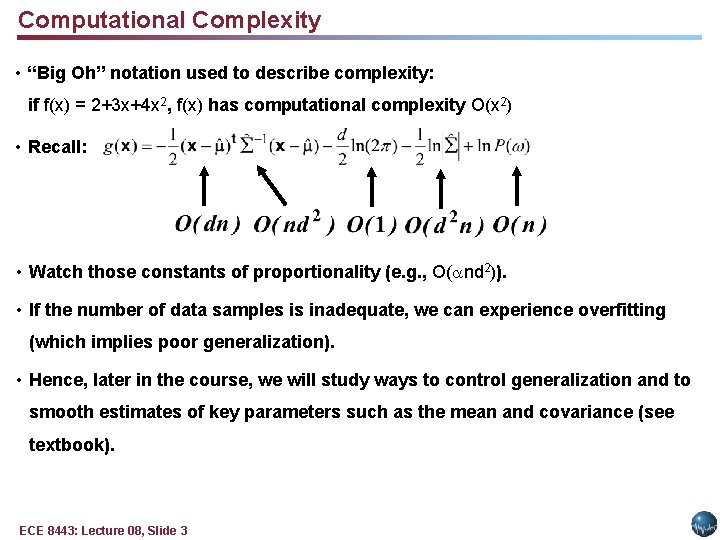
Computational Complexity • “Big Oh” notation used to describe complexity: if f(x) = 2+3 x+4 x 2, f(x) has computational complexity O(x 2) • Recall: • Watch those constants of proportionality (e. g. , O( nd 2)). • If the number of data samples is inadequate, we can experience overfitting (which implies poor generalization). • Hence, later in the course, we will study ways to control generalization and to smooth estimates of key parameters such as the mean and covariance (see textbook). ECE 8443: Lecture 08, Slide 3

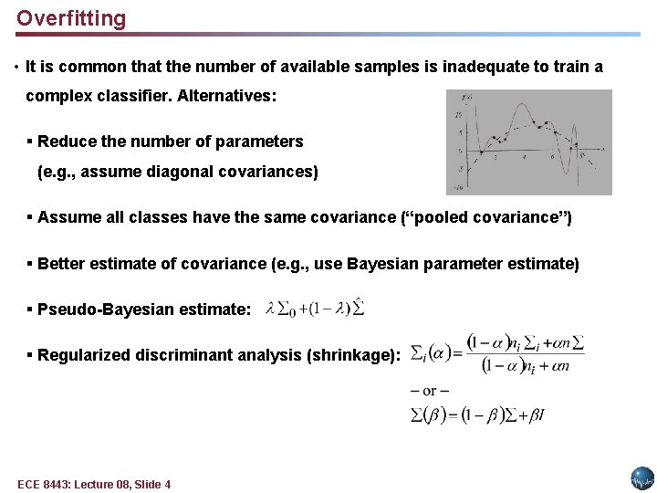
Overfitting • It is common that the number of available samples is inadequate to train a complex classifier. Alternatives: § Reduce the number of parameters (e. g. , assume diagonal covariances) § Assume all classes have the same covariance (“pooled covariance”) § Better estimate of covariance (e. g. , use Bayesian parameter estimate) § Pseudo-Bayesian estimate: § Regularized discriminant analysis (shrinkage): ECE 8443: Lecture 08, Slide 4

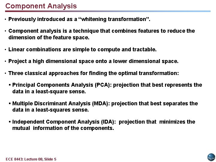
Component Analysis • Previously introduced as a “whitening transformation”. • Component analysis is a technique that combines features to reduce the dimension of the feature space. • Linear combinations are simple to compute and tractable. • Project a high dimensional space onto a lower dimensional space. • Three classical approaches for finding the optimal transformation: § Principal Components Analysis (PCA): projection that best represents the data in a least-square sense. § Multiple Discriminant Analysis (MDA): projection that best separates the data in a least-squares sense. § Independent Component Analysis (IDA): projection that minimizes the mutual information of the components. ECE 8443: Lecture 08, Slide 5

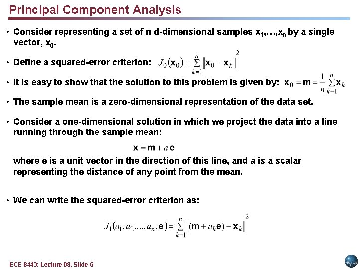
Principal Component Analysis • Consider representing a set of n d-dimensional samples x 1, …, xn by a single vector, x 0. • Define a squared-error criterion: • It is easy to show that the solution to this problem is given by: • The sample mean is a zero-dimensional representation of the data set. • Consider a one-dimensional solution in which we project the data into a line running through the sample mean: where e is a unit vector in the direction of this line, and a is a scalar representing the distance of any point from the mean. • We can write the squared-error criterion as: ECE 8443: Lecture 08, Slide 6

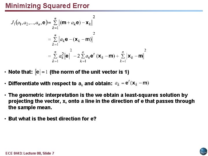
Minimizing Squared Error • Note that: (the norm of the unit vector is 1) • Differentiate with respect to ak and obtain: • The geometric interpretation is the we obtain a least-squares solution by projecting the vector, x, onto a line in the direction of e that passes through the sample mean. • But what is the best direction for e? ECE 8443: Lecture 08, Slide 7

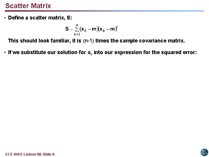
Scatter Matrix • Define a scatter matrix, S: This should look familiar, it is (n-1) times the sample covariance matrix. • If we substitute our solution for ak into our expression for the squared error: ECE 8443: Lecture 08, Slide 8

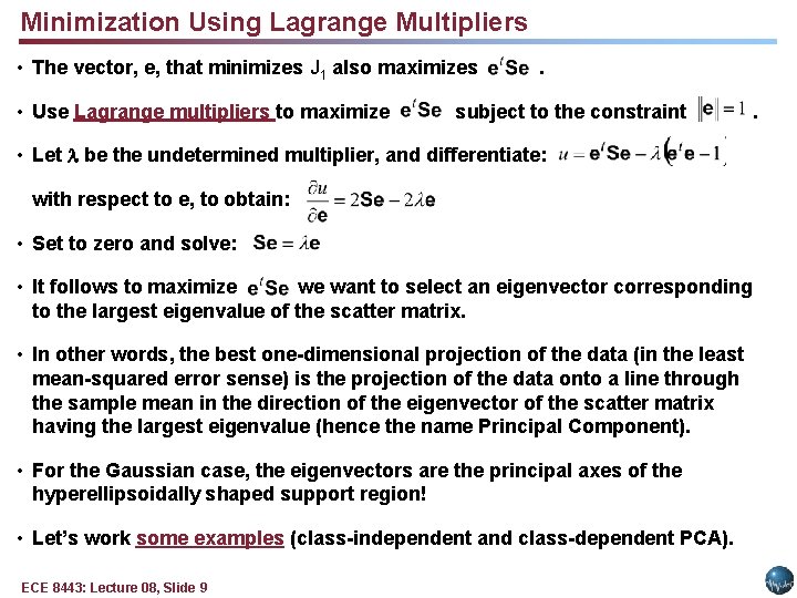
Minimization Using Lagrange Multipliers • The vector, e, that minimizes J 1 also maximizes • Use Lagrange multipliers to maximize . subject to the constraint • Let be the undetermined multiplier, and differentiate: with respect to e, to obtain: • Set to zero and solve: • It follows to maximize we want to select an eigenvector corresponding to the largest eigenvalue of the scatter matrix. • In other words, the best one-dimensional projection of the data (in the least mean-squared error sense) is the projection of the data onto a line through the sample mean in the direction of the eigenvector of the scatter matrix having the largest eigenvalue (hence the name Principal Component). • For the Gaussian case, the eigenvectors are the principal axes of the hyperellipsoidally shaped support region! • Let’s work some examples (class-independent and class-dependent PCA). ECE 8443: Lecture 08, Slide 9 .

Summary • The “curse of dimensionality. ” • Dimensionality and training data size. • Overfitting can be avoided by using weighted combinations of the pooled covariances and individual covariances. • Types of component analysis. • Principal component analysis: represents the data by minimizing the squared error (representing data in directions of greatest variance). • Example of class-independent and class-dependent analysis. • Insight into the important dimensions of your problem. • Next we will generalize PCA by introducing notions of discrimination. ECE 8443: Lecture 08, Slide 10