DifferentiationDiscrete Functions Electric Engineering Majors Authors Autar Kaw

Differentiation-Discrete Functions Electric Engineering Majors Authors: Autar Kaw, Sri Harsha Garapati http: //numericalmethods. eng. usf. edu Transforming Numerical Methods Education for STEM Undergraduates 10/19/2021 http: //numericalmethods. eng. usf. edu 1

Differentiation –Discrete Functions http: //numericalmethods. eng. usf. edu

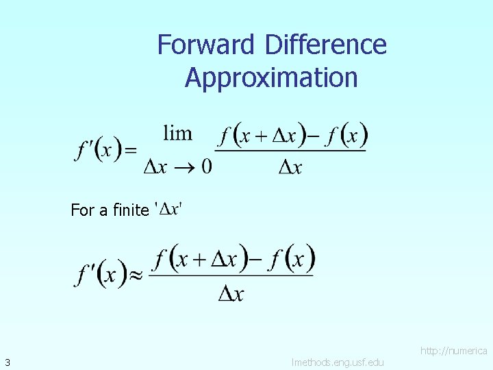
Forward Difference Approximation For a finite 3 lmethods. eng. usf. edu http: //numerica

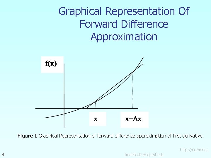
Graphical Representation Of Forward Difference Approximation Figure 1 Graphical Representation of forward difference approximation of first derivative. 4 lmethods. eng. usf. edu http: //numerica

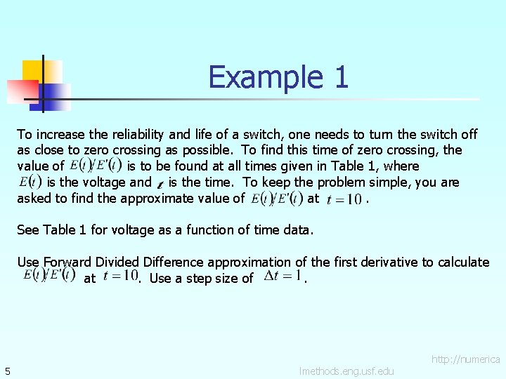
Example 1 To increase the reliability and life of a switch, one needs to turn the switch off as close to zero crossing as possible. To find this time of zero crossing, the value of is to be found at all times given in Table 1, where is the voltage and is the time. To keep the problem simple, you are asked to find the approximate value of at. See Table 1 for voltage as a function of time data. Use Forward Divided Difference approximation of the first derivative to calculate at. Use a step size of. 5 lmethods. eng. usf. edu http: //numerica

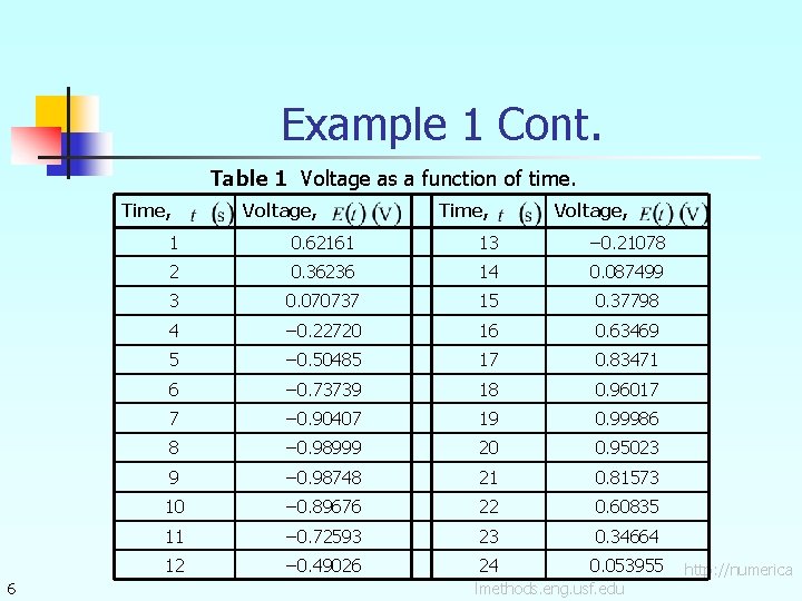
Example 1 Cont. Table 1 Voltage as a function of time. Time, 6 Voltage, Time, Voltage, 1 0. 62161 13 − 0. 21078 2 0. 36236 14 0. 087499 3 0. 070737 15 0. 37798 4 − 0. 22720 16 0. 63469 5 − 0. 50485 17 0. 83471 6 − 0. 73739 18 0. 96017 7 − 0. 90407 19 0. 99986 8 − 0. 98999 20 0. 95023 9 − 0. 98748 21 0. 81573 10 − 0. 89676 22 0. 60835 11 − 0. 72593 23 0. 34664 12 − 0. 49026 24 0. 053955 lmethods. eng. usf. edu http: //numerica

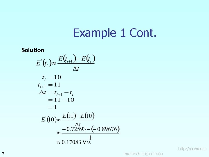
Example 1 Cont. Solution 7 lmethods. eng. usf. edu http: //numerica

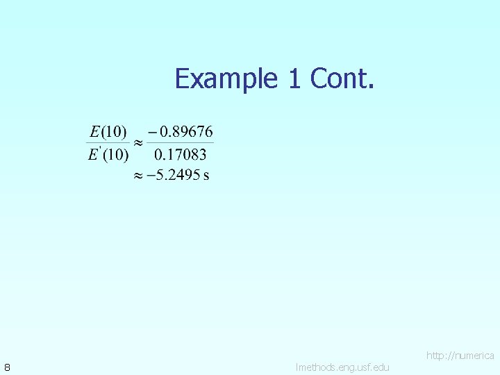
Example 1 Cont. 8 lmethods. eng. usf. edu http: //numerica

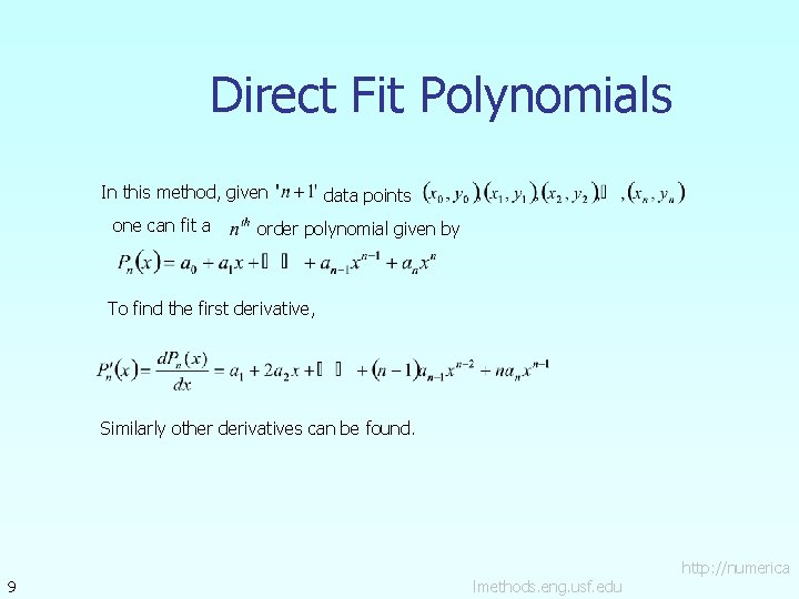
Direct Fit Polynomials In this method, given one can fit a data points order polynomial given by To find the first derivative, Similarly other derivatives can be found. 9 lmethods. eng. usf. edu http: //numerica

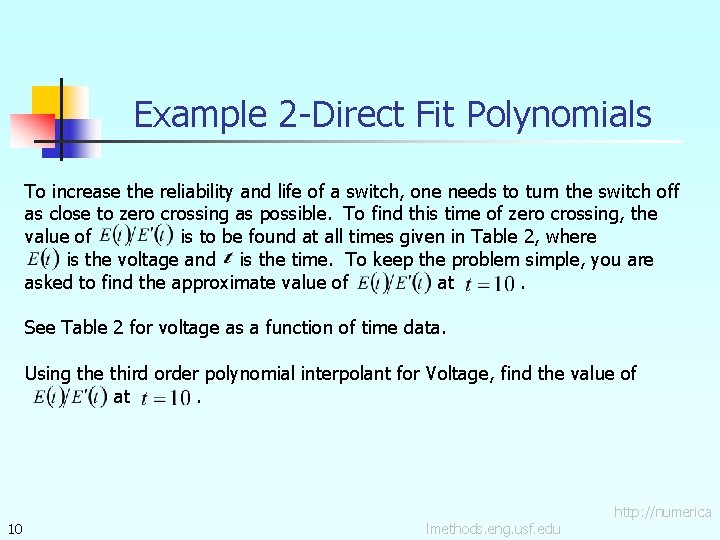
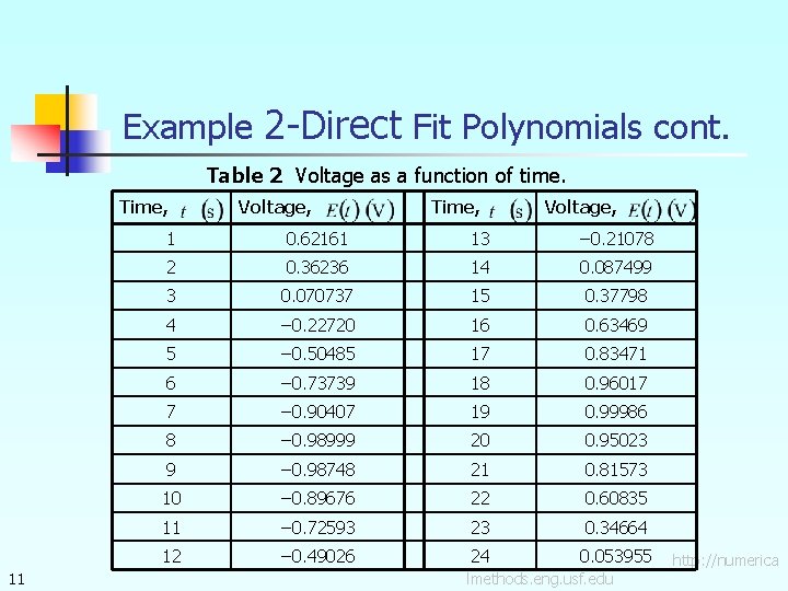
Example 2 -Direct Fit Polynomials To increase the reliability and life of a switch, one needs to turn the switch off as close to zero crossing as possible. To find this time of zero crossing, the value of is to be found at all times given in Table 2, where is the voltage and is the time. To keep the problem simple, you are asked to find the approximate value of at. See Table 2 for voltage as a function of time data. Using the third order polynomial interpolant for Voltage, find the value of at. 10 lmethods. eng. usf. edu http: //numerica

Example 2 -Direct Fit Polynomials cont. Table 2 Voltage as a function of time. Time, 11 Voltage, Time, Voltage, 1 0. 62161 13 − 0. 21078 2 0. 36236 14 0. 087499 3 0. 070737 15 0. 37798 4 − 0. 22720 16 0. 63469 5 − 0. 50485 17 0. 83471 6 − 0. 73739 18 0. 96017 7 − 0. 90407 19 0. 99986 8 − 0. 98999 20 0. 95023 9 − 0. 98748 21 0. 81573 10 − 0. 89676 22 0. 60835 11 − 0. 72593 23 0. 34664 12 − 0. 49026 24 0. 053955 lmethods. eng. usf. edu http: //numerica

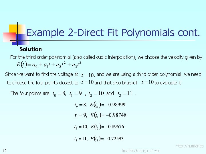
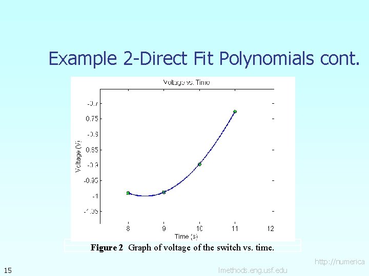
Example 2 -Direct Fit Polynomials cont. Solution For the third order polynomial (also called cubic interpolation), we choose the velocity given by Since we want to find the voltage at , and we are using a third order polynomial, we need and that also bracket to choose the four points closest to The four points are 12 , , and to evaluate it. . lmethods. eng. usf. edu http: //numerica

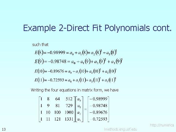
Example 2 -Direct Fit Polynomials cont. such that Writing the four equations in matrix form, we have 13 lmethods. eng. usf. edu http: //numerica

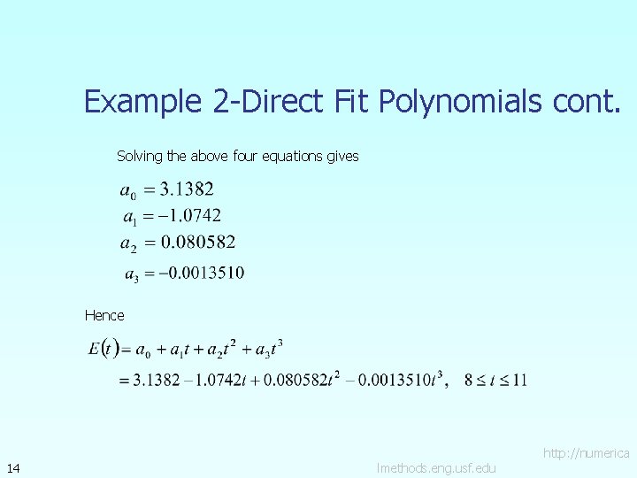
Example 2 -Direct Fit Polynomials cont. Solving the above four equations gives Hence 14 lmethods. eng. usf. edu http: //numerica

Example 2 -Direct Fit Polynomials cont. Figure 2 Graph of voltage of the switch vs. time. 15 lmethods. eng. usf. edu http: //numerica

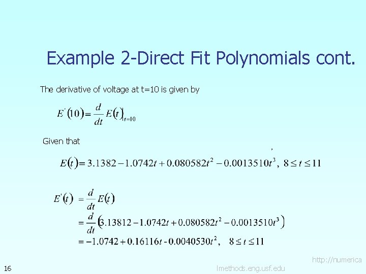
Example 2 -Direct Fit Polynomials cont. The derivative of voltage at t=10 is given by Given that 16 , lmethods. eng. usf. edu http: //numerica

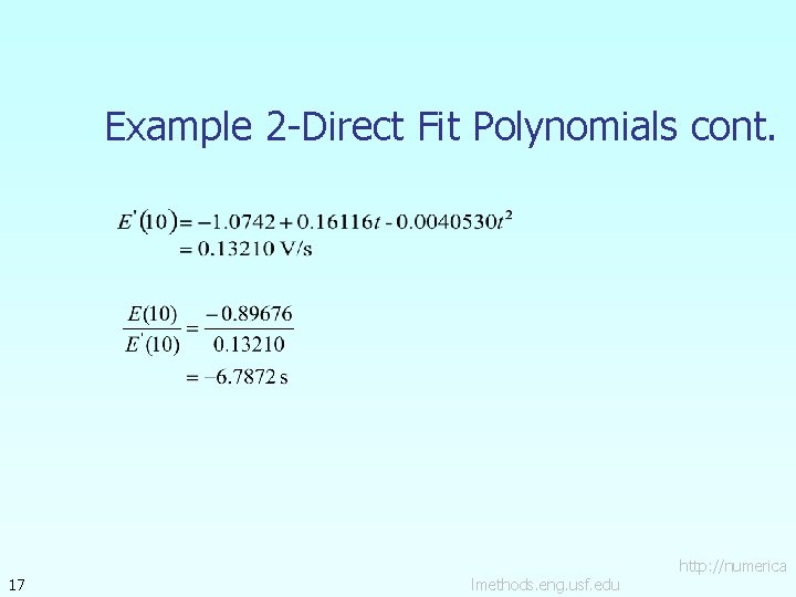
Example 2 -Direct Fit Polynomials cont. 17 lmethods. eng. usf. edu http: //numerica

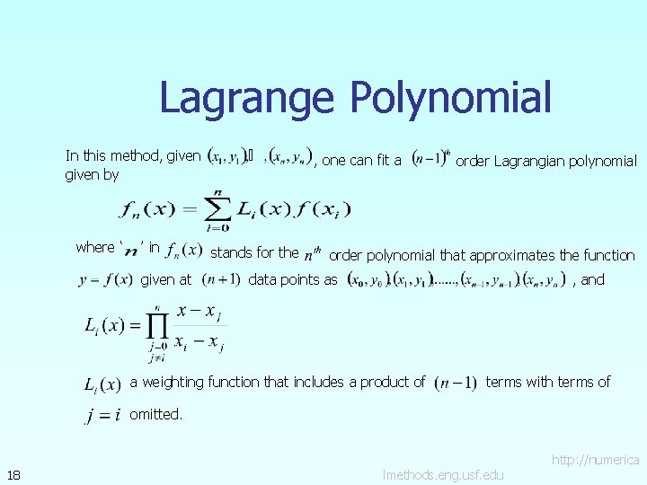
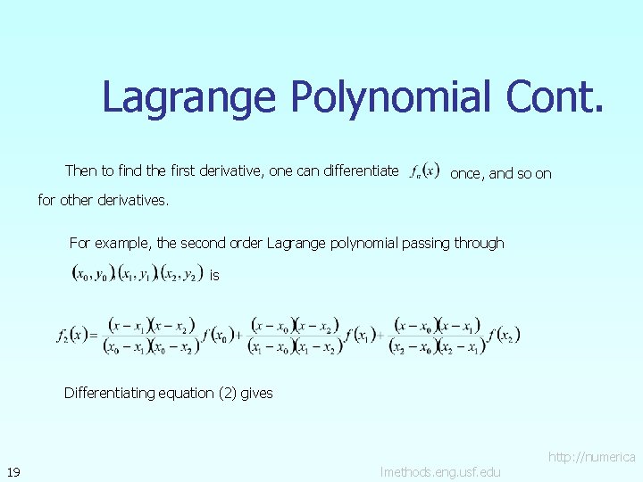
Lagrange Polynomial In this method, given by where ‘ ’ in given at , one can fit a stands for the order Lagrangian polynomial order polynomial that approximates the function data points as , and a weighting function that includes a product of terms with terms of omitted. 18 lmethods. eng. usf. edu http: //numerica

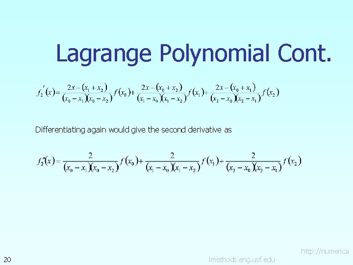
Lagrange Polynomial Cont. Then to find the first derivative, one can differentiate once, and so on for other derivatives. For example, the second order Lagrange polynomial passing through is Differentiating equation (2) gives 19 lmethods. eng. usf. edu http: //numerica

Lagrange Polynomial Cont. Differentiating again would give the second derivative as 20 lmethods. eng. usf. edu http: //numerica

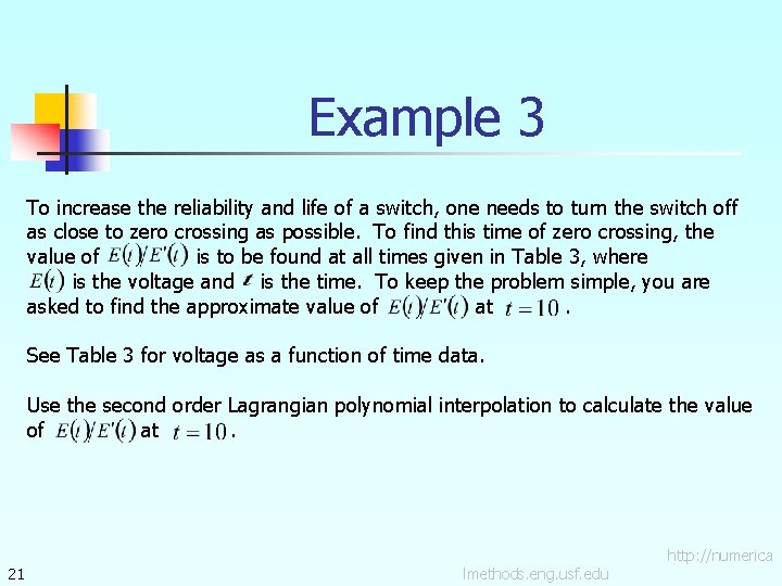
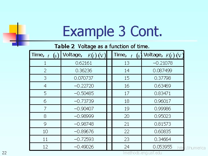
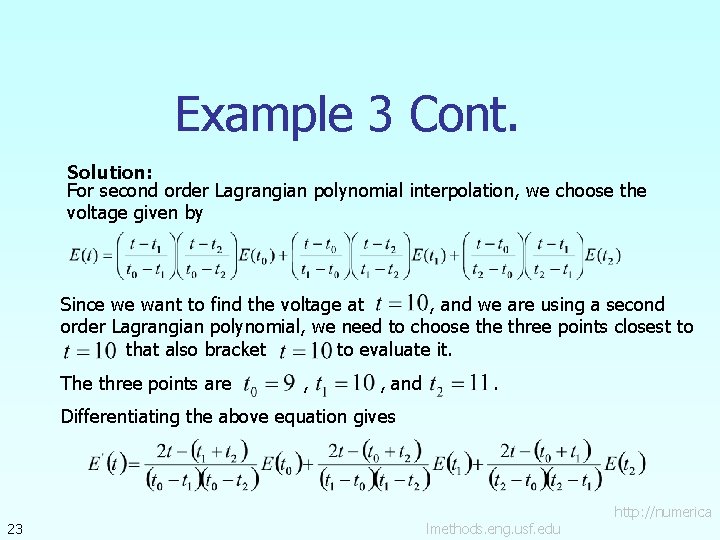
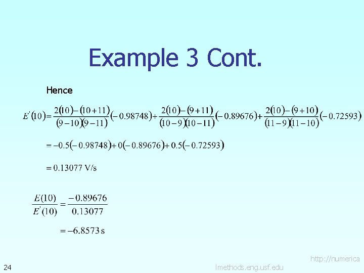
Example 3 To increase the reliability and life of a switch, one needs to turn the switch off as close to zero crossing as possible. To find this time of zero crossing, the value of is to be found at all times given in Table 3, where is the voltage and is the time. To keep the problem simple, you are asked to find the approximate value of at. See Table 3 for voltage as a function of time data. Use the second order Lagrangian polynomial interpolation to calculate the value of at. 21 lmethods. eng. usf. edu http: //numerica

Example 3 Cont. Table 2 Voltage as a function of time. Time, 22 Voltage, Time, Voltage, 1 0. 62161 13 − 0. 21078 2 0. 36236 14 0. 087499 3 0. 070737 15 0. 37798 4 − 0. 22720 16 0. 63469 5 − 0. 50485 17 0. 83471 6 − 0. 73739 18 0. 96017 7 − 0. 90407 19 0. 99986 8 − 0. 98999 20 0. 95023 9 − 0. 98748 21 0. 81573 10 − 0. 89676 22 0. 60835 11 − 0. 72593 23 0. 34664 12 − 0. 49026 24 0. 053955 lmethods. eng. usf. edu http: //numerica

Example 3 Cont. Solution: For second order Lagrangian polynomial interpolation, we choose the voltage given by Since we want to find the voltage at , and we are using a second order Lagrangian polynomial, we need to choose three points closest to that also bracket to evaluate it. The three points are , , and . Differentiating the above equation gives 23 lmethods. eng. usf. edu http: //numerica

Example 3 Cont. Hence 24 lmethods. eng. usf. edu http: //numerica

Additional Resources For all resources on this topic such as digital audiovisual lectures, primers, textbook chapters, multiple-choice tests, worksheets in MATLAB, MATHEMATICA, Math. Cad and MAPLE, blogs, related physical problems, please visit http: //numericalmethods. eng. usf. edu/topics/discrete_02 dif. html

THE END http: //numericalmethods. eng. usf. edu