DifferentiationDiscrete Functions Civil Engineering Majors Authors Autar Kaw

Differentiation-Discrete Functions Civil Engineering Majors Authors: Autar Kaw, Sri Harsha Garapati http: //numericalmethods. eng. usf. edu Transforming Numerical Methods Education for STEM Undergraduates 9/18/2021 http: //numericalmethods. eng. usf. edu 1

Differentiation –Discrete Functions http: //numericalmethods. eng. usf. edu

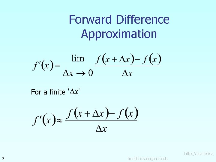
Forward Difference Approximation For a finite 3 lmethods. eng. usf. edu http: //numerica

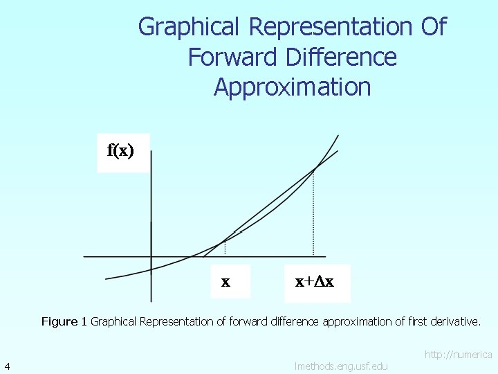
Graphical Representation Of Forward Difference Approximation Figure 1 Graphical Representation of forward difference approximation of first derivative. 4 lmethods. eng. usf. edu http: //numerica

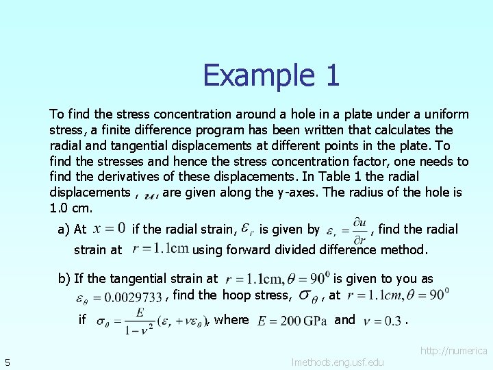
Example 1 To find the stress concentration around a hole in a plate under a uniform stress, a finite difference program has been written that calculates the radial and tangential displacements at different points in the plate. To find the stresses and hence the stress concentration factor, one needs to find the derivatives of these displacements. In Table 1 the radial displacements , , are given along the y-axes. The radius of the hole is 1. 0 cm. a) At strain at if the radial strain, is given by using forward divided difference method. b) If the tangential strain at , find the hoop stress, if 5 , find the radial , where is given to you as , at and lmethods. eng. usf. edu . http: //numerica

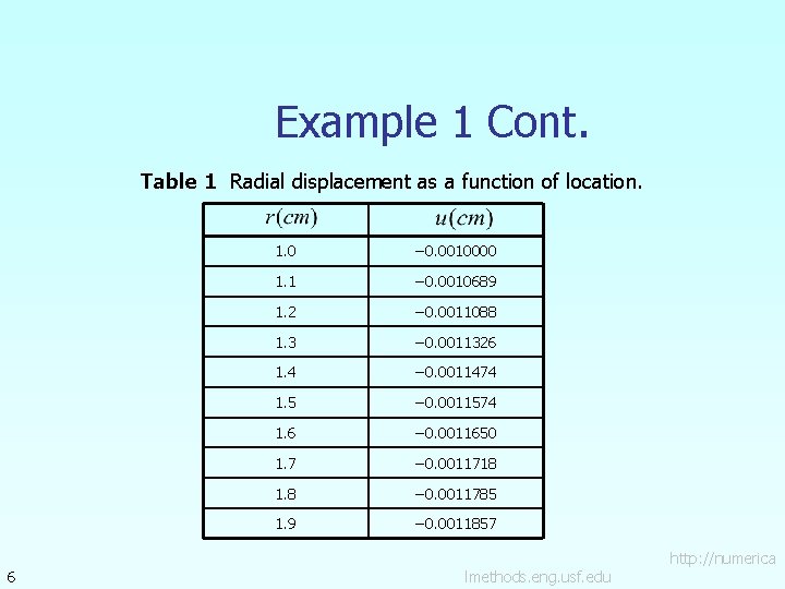
Example 1 Cont. Table 1 Radial displacement as a function of location. 6 1. 0 − 0. 0010000 1. 1 − 0. 0010689 1. 2 − 0. 0011088 1. 3 − 0. 0011326 1. 4 − 0. 0011474 1. 5 − 0. 0011574 1. 6 − 0. 0011650 1. 7 − 0. 0011718 1. 8 − 0. 0011785 1. 9 − 0. 0011857 lmethods. eng. usf. edu http: //numerica

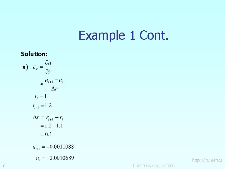
Example 1 Cont. Solution: a) 7 lmethods. eng. usf. edu http: //numerica

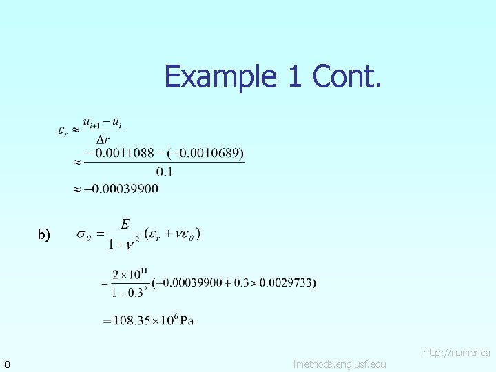
Example 1 Cont. b) 8 lmethods. eng. usf. edu http: //numerica

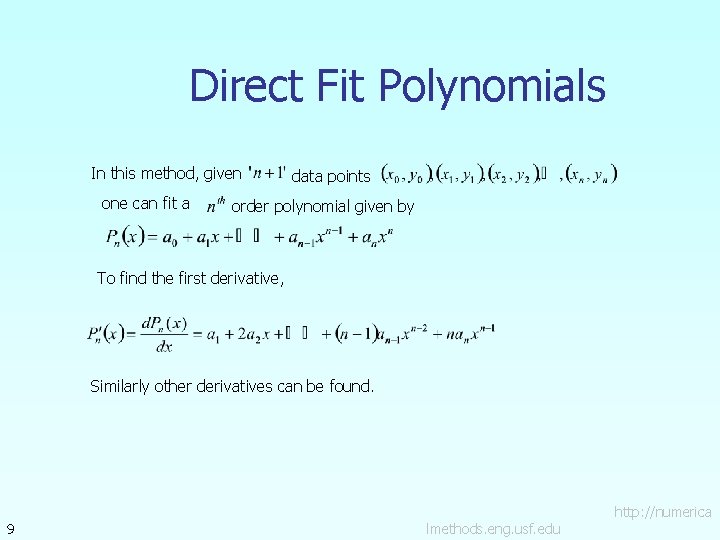
Direct Fit Polynomials In this method, given one can fit a data points order polynomial given by To find the first derivative, Similarly other derivatives can be found. 9 lmethods. eng. usf. edu http: //numerica

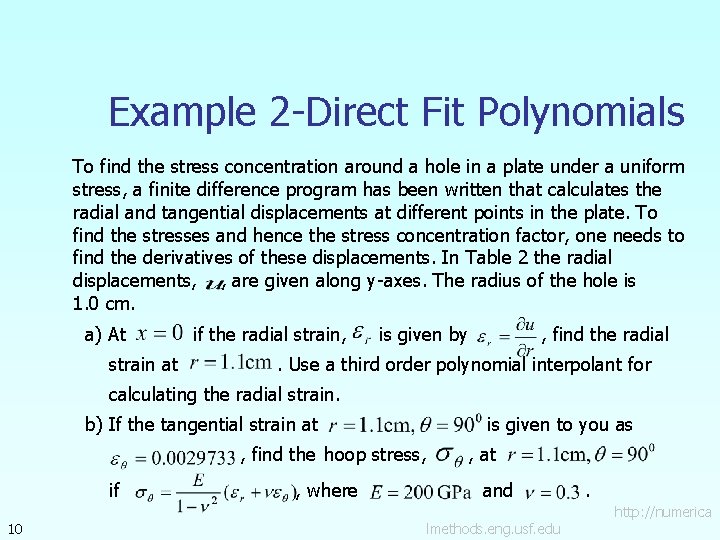
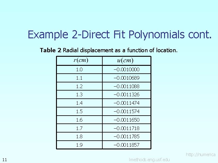
Example 2 -Direct Fit Polynomials To find the stress concentration around a hole in a plate under a uniform stress, a finite difference program has been written that calculates the radial and tangential displacements at different points in the plate. To find the stresses and hence the stress concentration factor, one needs to find the derivatives of these displacements. In Table 2 the radial displacements, , are given along y-axes. The radius of the hole is 1. 0 cm. a) At strain at if the radial strain, is given by , find the radial . Use a third order polynomial interpolant for calculating the radial strain. b) If the tangential strain at , find the hoop stress, if 10 , where is given to you as , at and lmethods. eng. usf. edu . http: //numerica

Example 2 -Direct Fit Polynomials cont. Table 2 Radial displacement as a function of location. 11 1. 0 − 0. 0010000 1. 1 − 0. 0010689 1. 2 − 0. 0011088 1. 3 − 0. 0011326 1. 4 − 0. 0011474 1. 5 − 0. 0011574 1. 6 − 0. 0011650 1. 7 − 0. 0011718 1. 8 − 0. 0011785 1. 9 − 0. 0011857 lmethods. eng. usf. edu http: //numerica

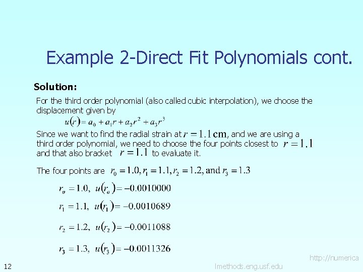
Example 2 -Direct Fit Polynomials cont. Solution: For the third order polynomial (also called cubic interpolation), we choose the displacement given by Since we want to find the radial strain at , and we are using a third order polynomial, we need to choose the four points closest to and that also bracket to evaluate it. The four points are 12 lmethods. eng. usf. edu http: //numerica

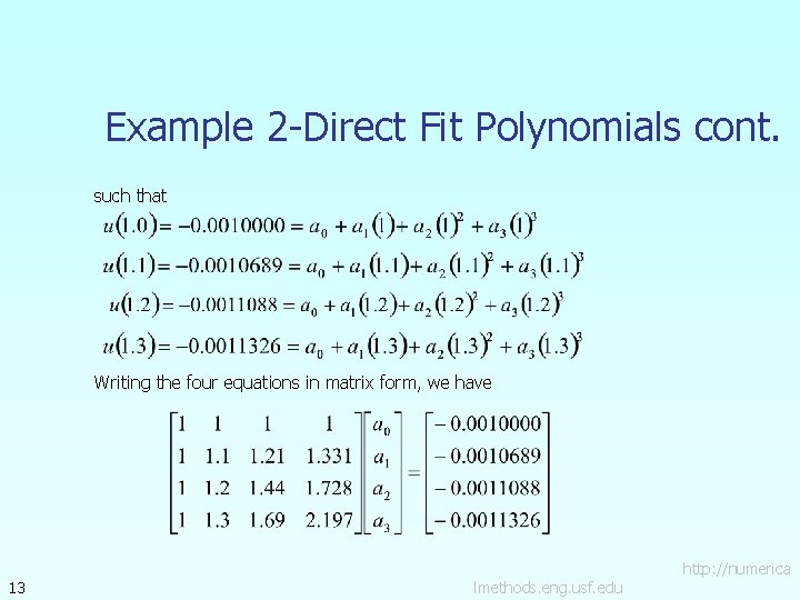
Example 2 -Direct Fit Polynomials cont. such that Writing the four equations in matrix form, we have 13 lmethods. eng. usf. edu http: //numerica

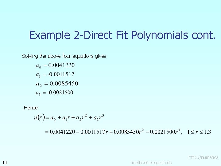
Example 2 -Direct Fit Polynomials cont. Solving the above four equations gives Hence 14 lmethods. eng. usf. edu http: //numerica

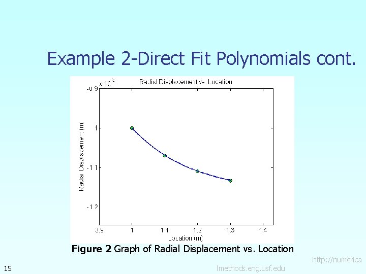
Example 2 -Direct Fit Polynomials cont. Figure 2 Graph of Radial Displacement vs. Location 15 lmethods. eng. usf. edu http: //numerica

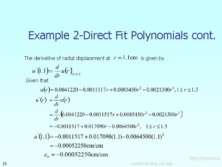
Example 2 -Direct Fit Polynomials cont. The derivative of radial displacement at is given by Given that 16 lmethods. eng. usf. edu http: //numerica

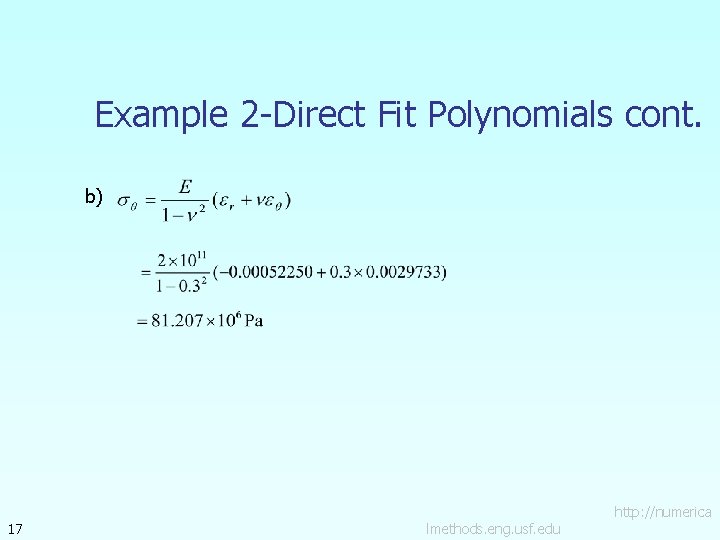
Example 2 -Direct Fit Polynomials cont. b) 17 lmethods. eng. usf. edu http: //numerica

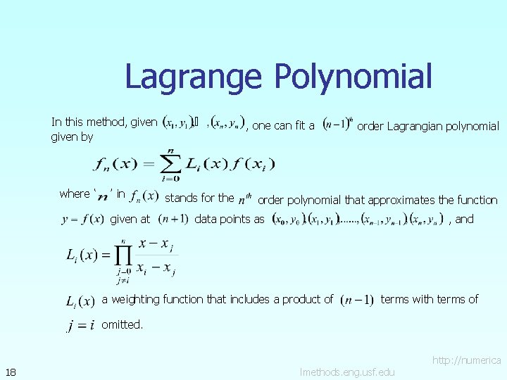
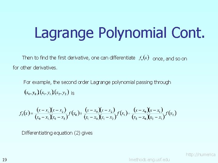
Lagrange Polynomial In this method, given by where ‘ ’ in given at , one can fit a stands for the order Lagrangian polynomial order polynomial that approximates the function data points as , and a weighting function that includes a product of terms with terms of omitted. 18 lmethods. eng. usf. edu http: //numerica

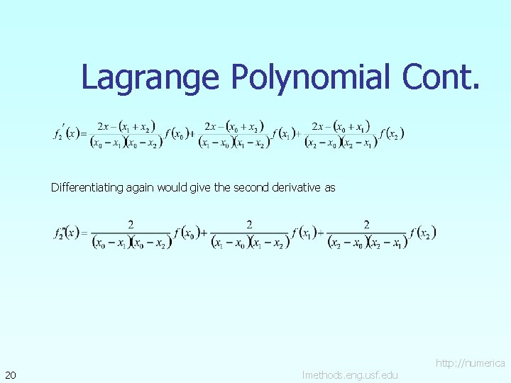
Lagrange Polynomial Cont. Then to find the first derivative, one can differentiate once, and so on for other derivatives. For example, the second order Lagrange polynomial passing through is Differentiating equation (2) gives 19 lmethods. eng. usf. edu http: //numerica

Lagrange Polynomial Cont. Differentiating again would give the second derivative as 20 lmethods. eng. usf. edu http: //numerica

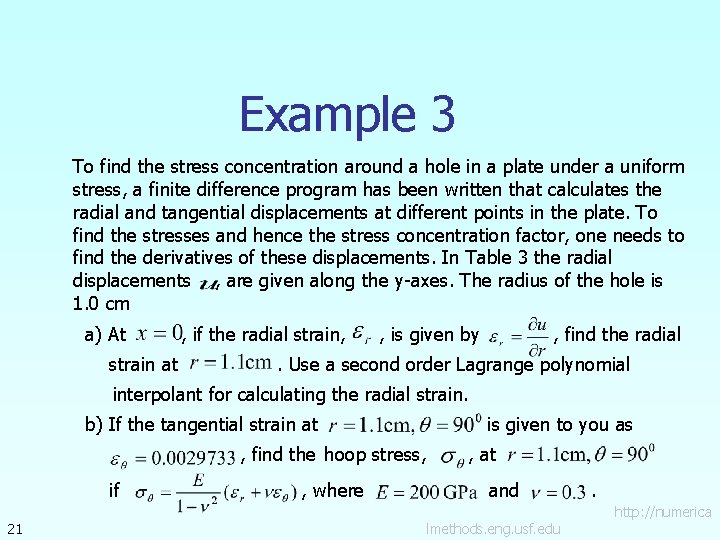
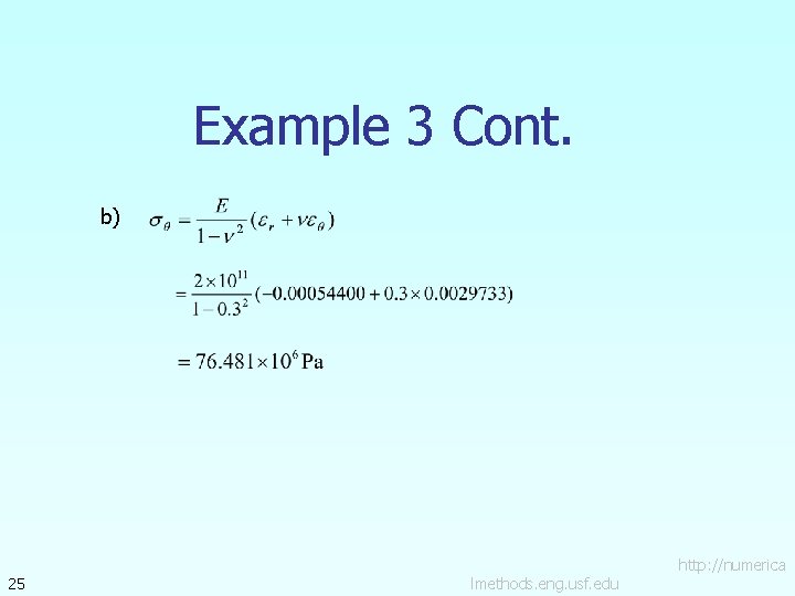
Example 3 To find the stress concentration around a hole in a plate under a uniform stress, a finite difference program has been written that calculates the radial and tangential displacements at different points in the plate. To find the stresses and hence the stress concentration factor, one needs to find the derivatives of these displacements. In Table 3 the radial displacements , are given along the y-axes. The radius of the hole is 1. 0 cm a) At strain at , if the radial strain, , is given by , find the radial . Use a second order Lagrange polynomial interpolant for calculating the radial strain. b) If the tangential strain at , find the hoop stress, if 21 , where is given to you as , at and lmethods. eng. usf. edu . http: //numerica

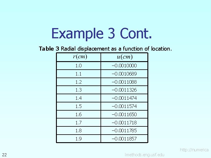
Example 3 Cont. Table 3 Radial displacement as a function of location. 22 1. 0 − 0. 0010000 1. 1 − 0. 0010689 1. 2 − 0. 0011088 1. 3 − 0. 0011326 1. 4 − 0. 0011474 1. 5 − 0. 0011574 1. 6 − 0. 0011650 1. 7 − 0. 0011718 1. 8 − 0. 0011785 1. 9 − 0. 0011857 lmethods. eng. usf. edu http: //numerica

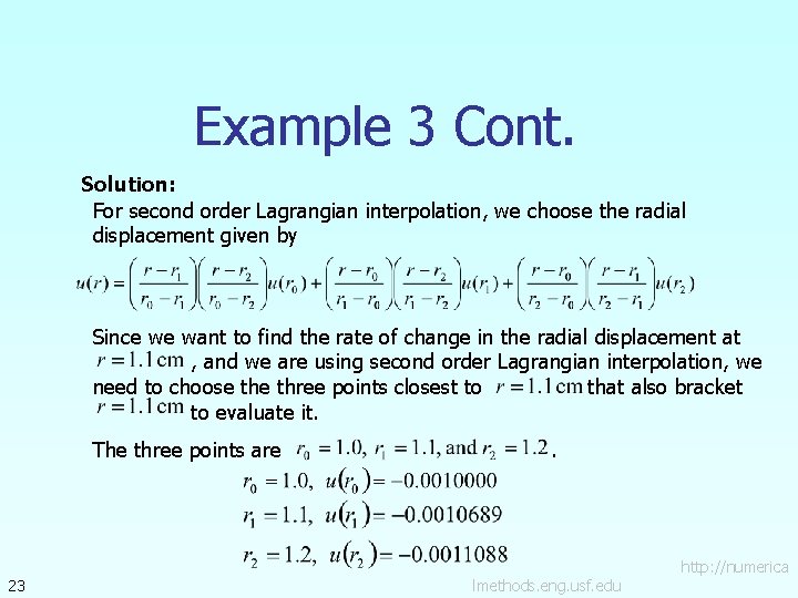
Example 3 Cont. Solution: For second order Lagrangian interpolation, we choose the radial displacement given by Since we want to find the rate of change in the radial displacement at , and we are using second order Lagrangian interpolation, we need to choose three points closest to that also bracket to evaluate it. The three points are 23 . lmethods. eng. usf. edu http: //numerica

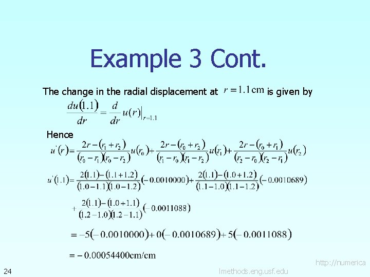
Example 3 Cont. The change in the radial displacement at is given by Hence 24 lmethods. eng. usf. edu http: //numerica

Example 3 Cont. b) 25 lmethods. eng. usf. edu http: //numerica

Additional Resources For all resources on this topic such as digital audiovisual lectures, primers, textbook chapters, multiple-choice tests, worksheets in MATLAB, MATHEMATICA, Math. Cad and MAPLE, blogs, related physical problems, please visit http: //numericalmethods. eng. usf. edu/topics/discrete_02 dif. html

THE END http: //numericalmethods. eng. usf. edu