Chapter Three The Standard Theory of International Trade

Chapter Three: The Standard Theory of International Trade

3. 1 introduction § The model introduces increasing opp. costs and tastes or demand preferences with community indifference curves. § Forces of demand supply determine the equilibrium-relative commodity price in each nation in the absence of trade under increasing costs and will indicate the commodity of comp-adv. for each nation. § Then see how with trade, each nation gains by specializing in production and export of the commodity with which it has comp-adv. and import with which it has comp-disadv.

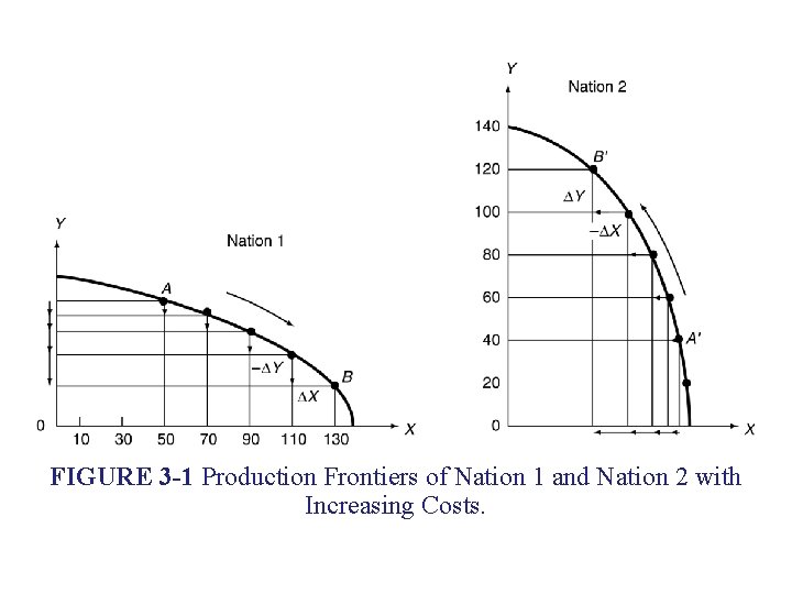
3. 2 Production Frontier with Increasing Costs § Increasing costs mean that the nation must give up more and more of one commodity to release just enough resources to produce each additional unit of another commodity. As a result, the PPF is concave. A. Illustration of Increasing Costs § In Fig. 3 -1, if nation 1 wants to increase output of X (point A), it should reduce output of Y by more and more units. § If nation 2 wants to increase output of Y (point A/), it should reduce output of X by more and more units § Thus, both nations face increasing costs in the production of the two commodities.

FIGURE 3 -1 Production Frontiers of Nation 1 and Nation 2 with Increasing Costs.

B. The Marginal Rate of Transformation (MRT) § The MRT of X for Y refers to the amount of Y that a nation must give up to produce additional unit of X. § It is another name for the opp. cost and is given by the slope of the production frontier at the point of production. § If the MRT of nation 1 at point A is ¼, this means that nation 1 must give up ¼ of a unit of Y to release just enough resources to produce one additional unit of X at this point. § If the MRT at point B is 1, a movement from A to B reflects the increasing opp. costs in producing more X

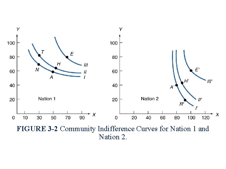
3. 3 Community Indifference Curves § A community indifference curve shows the various combinations of two commodities that yield equal satisfaction to the community. § Higher curves refer to greater satisfaction. A. Illustration of Community Indifference Curves § Fig. 3 -2 shows 3 hypothetical indifference curves for the two nations. They differ according to tastes. § Points A and N give equal satisfaction. § Points T and H refer to higher satisfaction

FIGURE 3 -2 Community Indifference Curves for Nation 1 and Nation 2.

B. The Marginal Rate of Substitution (MRS) § The MRS of X for Y in consumption refers to the amount of Y that a nation must give up for one extra unit of X and still remain on the same IC. § This is given by the (absolute) slope of the community IC at the point of consumption and declines as the nation moves down the curve. § The decline in MRS is a reflection of the fact that the more of X and less of Y a nation consumes, the more valuable Y becomes compared to X.

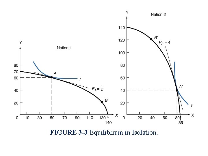
3. 4 Equilibrium in Isolation A. Illustration of Equilibrium in Isolation § Fig. 3 -3 combines the production frontiers and the community IC. § IC I is the highest IC curve that nation 1 can reach with its production frontier. Thus, it is in equil when it produces and consumes at point A in the absence of trade, or autarky. § There is only one point of tangency, or equilibrium.

FIGURE 3 -3 Equilibrium in Isolation.

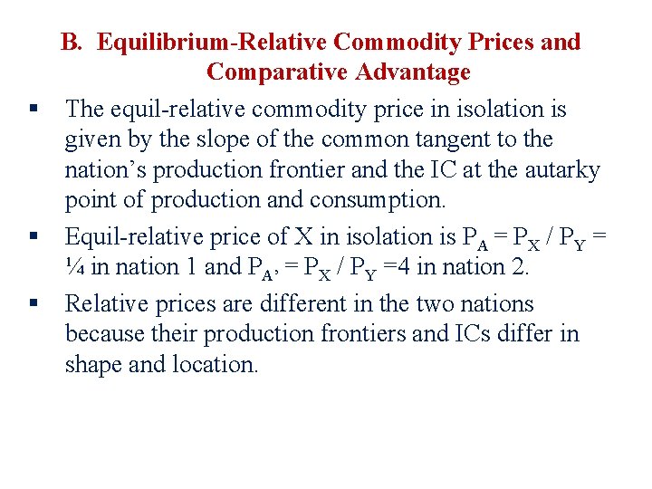
B. Equilibrium-Relative Commodity Prices and Comparative Advantage § The equil-relative commodity price in isolation is given by the slope of the common tangent to the nation’s production frontier and the IC at the autarky point of production and consumption. § Equil-relative price of X in isolation is PA = PX / PY = ¼ in nation 1 and PA’ = PX / PY =4 in nation 2. § Relative prices are different in the two nations because their production frontiers and ICs differ in shape and location.

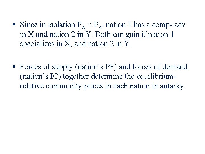
§ Since in isolation PA < PA’ nation 1 has a comp- adv in X and nation 2 in Y. Both can gain if nation 1 specializes in X, and nation 2 in Y. § Forces of supply (nation’s PF) and forces of demand (nation’s IC) together determine the equilibriumrelative commodity prices in each nation in autarky.

3. 5 The Basis for and the Gains from Trade with Increasing Costs A. Illustrations of the Basis for and the Gains from Trade with Increasing Costs § Starting from point A, as nation 1 specializes in X and moves down its PF, it incurs increasing opp. costs (as reflected in the increasing slope of the PF). § Starting from point A’, as nation 2 specializes in Y and moves upward its PF, it incurs increasing opp. costs (as reflected in the decline in slope of the PF). § Specialization in production continues until relative commodity prices become equal in the two nations.

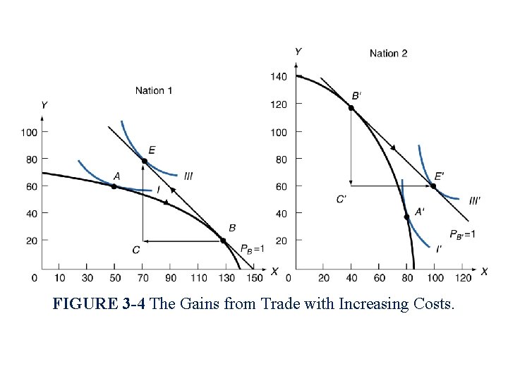
FIGURE 3 -4 The Gains from Trade with Increasing Costs.

§ The common relative price (slope) with trade will be somewhere between the pretrade relative prices of ¼ and 4, at the level at which trade is balanced. In figure 3 -4, this is PB = PB’ = 1. § With trade, nation 1 moves from A down to B. by exchanging 60 X for 60 Y with nation 2, nation 1 ends up consuming at E (70 X and 80 Y) on its IC III. § This is the highest level of satisfaction that nation 1 can reach with trade at PX/PY = 1. Thus, nation 1 gains 20 X & 20 Y from its no-trade equilibrium point. § Nation 2 moves from A’ to B’, and with trade of 60 Y for 60 X it ends up consuming at E’ (100 X and 60 Y). § Nation 2 gains 20 X & 20 Y from specialization/trade.

B. Equilibrium-Relative Commodity Prices with Trade (ERCPT) § The ERCPT is the common relative price in both nations at which trade is balanced, this is PB= PB’=1. § At this relative, the amount of X that nation 1 wants to export (60 X) equals the amount of X that nation 2 wants to import (60 X). Similarly for nation 2 and Y. § Any other relative price could not persist because trade would be unbalanced. § The greater the desire of nation 1 for Y and the weaker is nation 2’s desire for X, the closer the equil. price with trade will be to 1/4 and the smaller will be nation 1’s share of the gain.

§ Once equil-relative price with trade is determined, gains from trade will be known exactly and the model will be complete. § The equil-relative price of X with trade (PB= PB’=1) results in equal gains (20 X and 20 Y). § If the pretrade - relative price had been the same in both nations, there would be no comp-advantage or disadvantage in either nation, and no specialization in production or mutually beneficial trade would take place.

C. Incomplete Specialization § Under constant costs, both nations specialize completely in production of the commodity of their comparative advantage. § However, under increasing costs there is incomplete specialization in production in both nations. § That is, nation 1 continues producing Y (point B), and nation 2 continues producing X (point B’). § Reason: as nation 1 specializes in X, it incurs increasing opp. costs in production of X. Similarly, as nation 2 produces more Y, it incurs opp. costs in Y (implying decreasing opp. costs of X).

§ With specialization, relative prices move toward each other until they are identical in both nations. § At this point, it does not pay for either nation to continue expanding production of the commodity of its comparative advantage. § This occurs before either nation has completely specialized in production. § In figure 3 -4, before nation 1 or nation 2 has completely specialized in production.

D. Small –Country Case with Increasing Costs § Under constant costs, the small country completely specializes in the production of the commodity of its comparative advantage, but the large country doesn’t § However, under increasing costs, we find incomplete specialization even in the small country case. § Assume nation 1 is the small country. § With no trade, nation 1 at equil. at point A. § Suppose the equil-relative price of X on world market is 1 (PW=1), and not affected by trade with nation 1. § Since the pretrade relative price of X in nation 1 is PA=1/4 is lower than world price, it has comparative advantage in the production of X.

§ With trade, nation 1 specializes in X until it reaches point B where PB=1=PW § Even though nation 1 is a small country, it doesn’t completely specialize in X (as under constant costs). § By exchanging 60 X for 60 Y, nation 1 reaches point E and gains 20 X and 20 Y (compared to autarky; A). § The only difference from the case discussed before is that nation 1 doesn’t affect relative prices in nation 2. § Nation 1 captures all the benefits from trade.

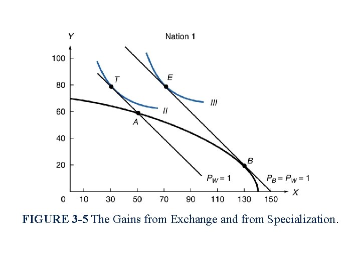
E. The Gains from Exchange and Specialization § A nation’s gains from trade arise from exchange and specialization. § Fig 3 -5 shows this breakdown for the small nation 1 § Suppose nation 1 could not specialize in X with trade and continued produce at A, where MRT=1/4 § Starting from A, nation 1 could export 20 X in exchange for 20 Y at PW =1 and end up at point T. § Although it consumes less of X and more of Y (at T) it is better off than it was in autarky because it is on higher indifference curve. § Movement from A to T in consumption measures the gain from exchange.

FIGURE 3 -5 The Gains from Exchange and from Specialization.

§ If subsequently nation 1 also specialized in X and produced at B, it could then exchange 60 X for 60 Y with the rest of the world and consume at E. § The movement from T to E in consumption measures the gains from specialization in production. § In sum, the movement from A (on IC I) to T (on IC II) made possible by exchange only. § The movement from T (on IC II) to E (on IC III) made possible by specialization in production. § Note that nation 1 is not in equil at point A with trade because MRT < PW. To be in equil in production, it should expand production of X until it reaches point B, where PB = PW =1