CHAPTER 24 MRPP Multiresponse Permutation Procedures and Related

CHAPTER 24 MRPP (Multi-response Permutation Procedures) and Related Techniques Tables, Figures, and Equations From: Mc. Cune, B. & J. B. Grace. 2002. Analysis of Ecological Communities. Mj. M Software Design, Gleneden Beach, Oregon http: //www. pcord. com

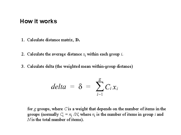
How it works 1. Calculate distance matrix, D. 2. Calculate the average distance xi within each group i. 3. Calculate delta (the weighted mean within-group distance) for g groups, where C is a weight that depends on the number of items in the groups (normally Ci = ni /N, where ni is the number of items in group i and N is the total number of items).

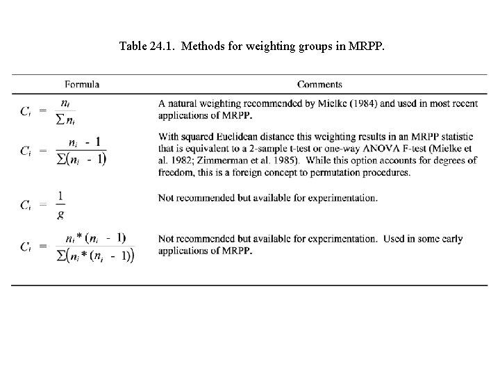
Table 24. 1. Methods for weighting groups in MRPP.

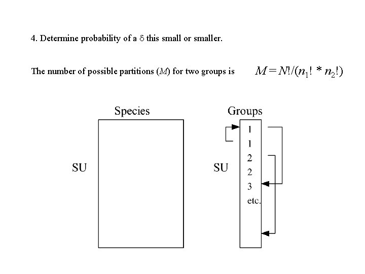
4. Determine probability of a this small or smaller. The number of possible partitions (M) for two groups is M = N!/(n 1! * n 2!)

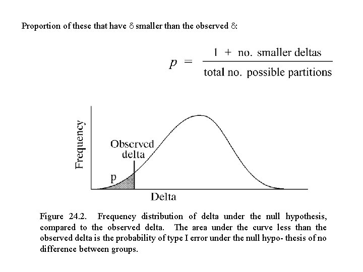
Proportion of these that have smaller than the observed : Figure 24. 2. Frequency distribution of delta under the null hypothesis, compared to the observed delta. The area under the curve less than the observed delta is the probability of type I error under the null hypo- thesis of no difference between groups.

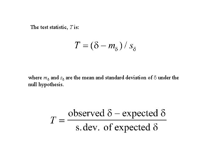
The test statistic, T is: where m and s are the mean and standard deviation of under the null hypothesis.

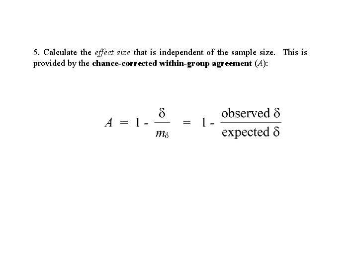
5. Calculate the effect size that is independent of the sample size. This is provided by the chance-corrected within-group agreement (A):

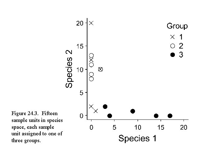
Figure 24. 3. Fifteen sample units in species space, each sample unit assigned to one of three groups.

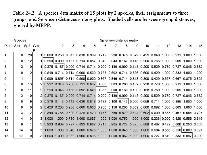
Table 24. 2. A species data matrix of 15 plots by 2 species, their assignments to three groups, and Sørensen distances among plots. Shaded cells are between-group distances, ignored by MRPP.

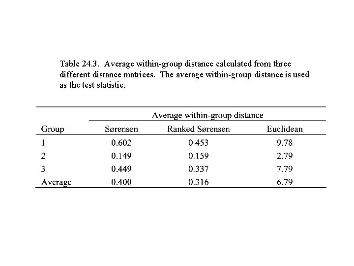
Table 24. 3. Average within-group distance calculated from three different distance matrices. The average within-group distance is used as the test statistic.

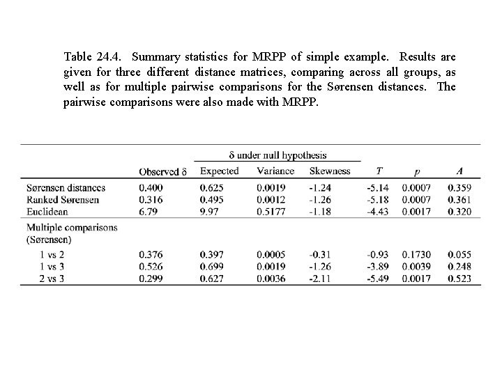
Table 24. 4. Summary statistics for MRPP of simple example. Results are given for three different distance matrices, comparing across all groups, as well as for multiple pairwise comparisons for the Sørensen distances. The pairwise comparisons were also made with MRPP.

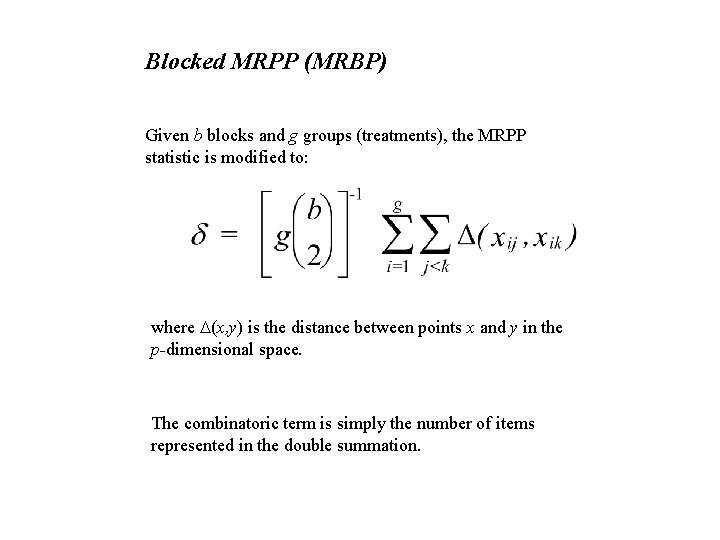
Blocked MRPP (MRBP) Given b blocks and g groups (treatments), the MRPP statistic is modified to: where D(x, y) is the distance between points x and y in the p-dimensional space. The combinatoric term is simply the number of items represented in the double summation.

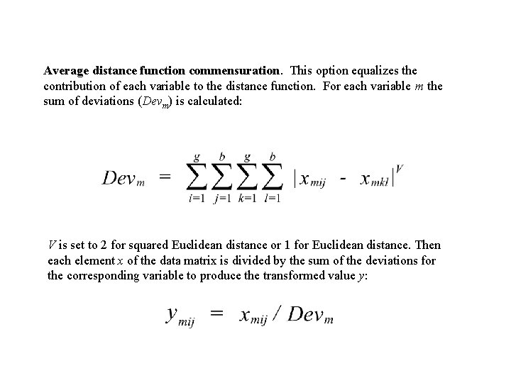
Average distance function commensuration. This option equalizes the contribution of each variable to the distance function. For each variable m the sum of deviations (Devm) is calculated: V is set to 2 for squared Euclidean distance or 1 for Euclidean distance. Then each element x of the data matrix is divided by the sum of the deviations for the corresponding variable to produce the transformed value y:

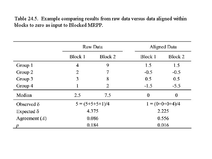
Table 24. 5. Example comparing results from raw data versus data aligned within blocks to zero as input to Blocked MRPP.

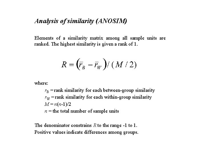
Analysis of similarity (ANOSIM) Elements of a similarity matrix among all sample units are ranked. The highest similarity is given a rank of 1. where: r. B = rank similarity for each between-group similarity r. W = rank similarity for each within-group similarity M = n(n-1)/2 n = the total number of sample units The denominator constrains R to the range -1 to 1. Positive values indicate differences among groups.

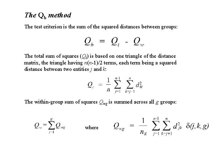
The Qb method The test criterion is the sum of the squared distances between groups: The total sum of squares (Qt) is based on one triangle of the distance matrix, the triangle having n(n-1)/2 terms, each term being a squared distance between two entities j and k: The within-group sum of squares Qwg is summed across all g groups: where

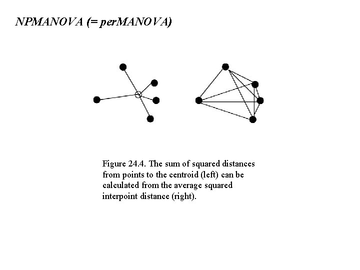
NPMANOVA (= per. MANOVA) Figure 24. 4. The sum of squared distances from points to the centroid (left) can be calculated from the average squared interpoint distance (right).

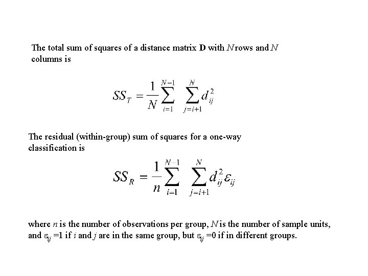
The total sum of squares of a distance matrix D with N rows and N columns is The residual (within-group) sum of squares for a one-way classification is where n is the number of observations per group, N is the number of sample units, and ij =1 if i and j are in the same group, but ij =0 if in different groups.

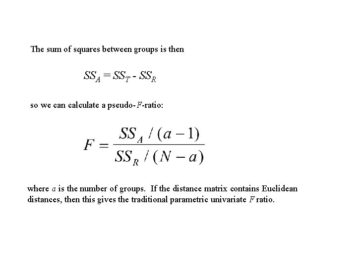
The sum of squares between groups is then SSA = SST - SSR so we can calculate a pseudo-F-ratio: where a is the number of groups. If the distance matrix contains Euclidean distances, then this gives the traditional parametric univariate F ratio.

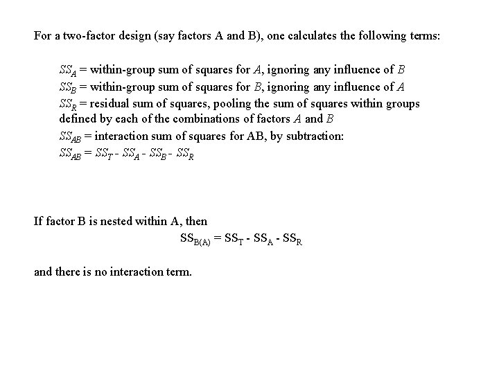
For a two-factor design (say factors A and B), one calculates the following terms: SSA = within-group sum of squares for A, ignoring any influence of B SSB = within-group sum of squares for B, ignoring any influence of A SSR = residual sum of squares, pooling the sum of squares within groups defined by each of the combinations of factors A and B SSAB = interaction sum of squares for AB, by subtraction: SSAB = SST - SSA - SSB - SSR If factor B is nested within A, then SSB(A) = SST - SSA - SSR and there is no interaction term.