Chapter 2 Fourier Transform and Spectra Topics Rectangular

Chapter 2 Fourier Transform and Spectra Topics: Ø Rectangular and Triangular Pulses Ø Spectrum of Rectangular, Triangular Pulses Ø Convolution Ø Spectrum by Convolution Huseyin Bilgekul Eeng 360 Communication Systems I Department of Electrical and Electronic Engineering Eastern Mediterranean University 1

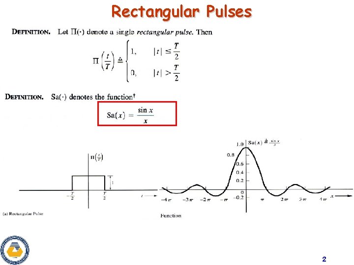
Rectangular Pulses 2

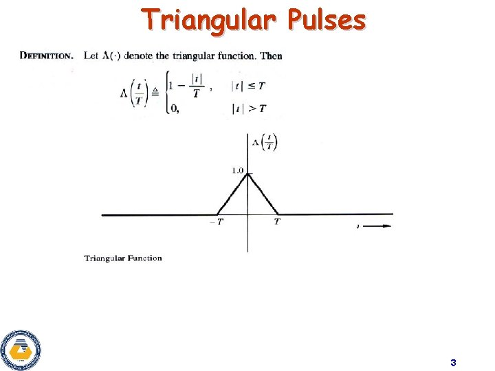
Triangular Pulses 3

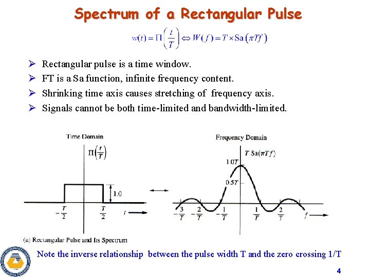
Spectrum of a Rectangular Pulse Ø Ø Rectangular pulse is a time window. FT is a Sa function, infinite frequency content. Shrinking time axis causes stretching of frequency axis. Signals cannot be both time-limited and bandwidth-limited. Note the inverse relationship between the pulse width T and the zero crossing 1/T 4

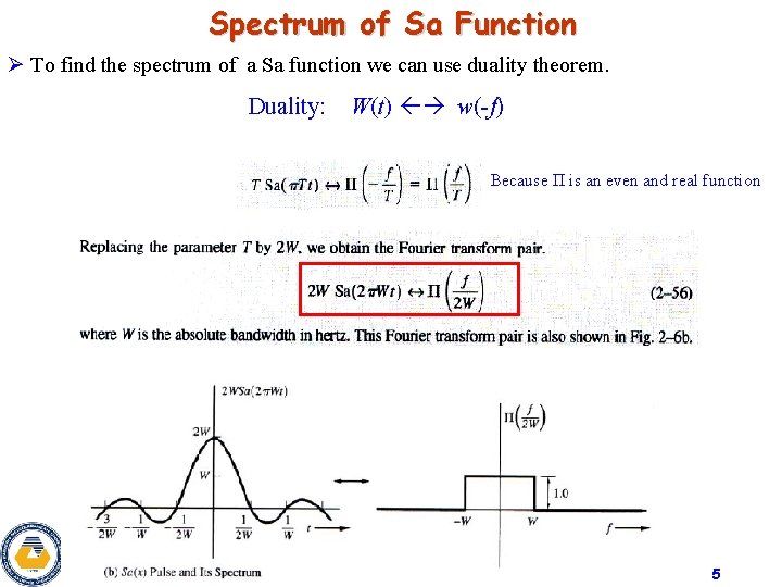
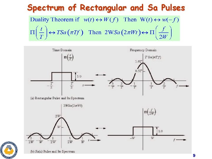
Spectrum of Sa Function Ø To find the spectrum of a Sa function we can use duality theorem. Duality: W(t) w(-f) Because Π is an even and real function 5

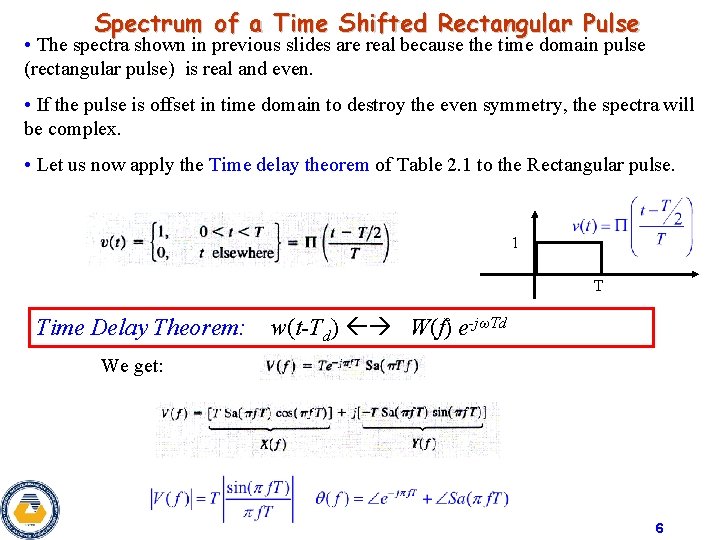
Spectrum of a Time Shifted Rectangular Pulse • The spectra shown in previous slides are real because the time domain pulse (rectangular pulse) is real and even. • If the pulse is offset in time domain to destroy the even symmetry, the spectra will be complex. • Let us now apply the Time delay theorem of Table 2. 1 to the Rectangular pulse. 1 T Time Delay Theorem: w(t-Td) W(f) e-jωTd We get: 6

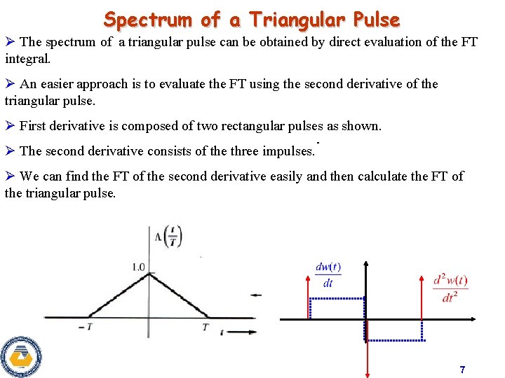
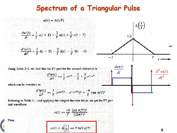
Spectrum of a Triangular Pulse Ø The spectrum of a triangular pulse can be obtained by direct evaluation of the FT integral. Ø An easier approach is to evaluate the FT using the second derivative of the triangular pulse. Ø First derivative is composed of two rectangular pulses as shown. Ø The second derivative consists of the three impulses. Ø We can find the FT of the second derivative easily and then calculate the FT of the triangular pulse. 7

Spectrum of a Triangular Pulse 8

Spectrum of Rectangular and Sa Pulses 9

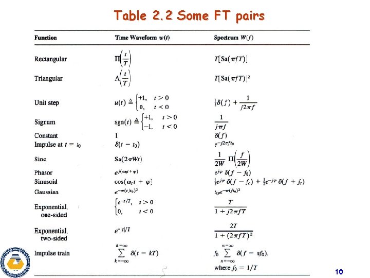
Table 2. 2 Some FT pairs 10

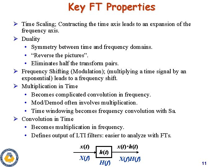
Key FT Properties Ø Time Scaling; Contracting the time axis leads to an expansion of the frequency axis. Ø Duality • Symmetry between time and frequency domains. • “Reverse the pictures”. • Eliminates half the transform pairs. Ø Frequency Shifting (Modulation); (multiplying a time signal by an exponential) leads to a frequency shift. Ø Multiplication in Time • Becomes complicated convolution in frequency. • Mod/Demod often involves multiplication. • Time windowing becomes frequency convolution with Sa. Ø Convolution in Time • Becomes multiplication in frequency. • Defines output of LTI filters: easier to analyze with FTs. x(t) X(f) h(t) H(f) x(t)*h(t) X(f)H(f) 11

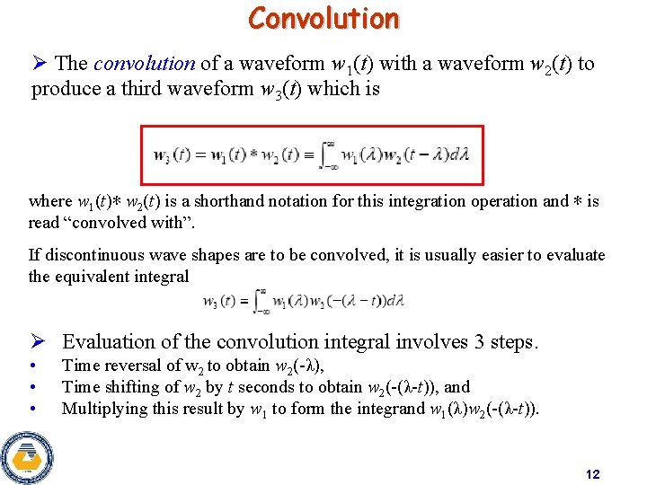
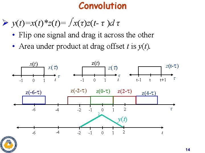
Convolution Ø The convolution of a waveform w 1(t) with a waveform w 2(t) to produce a third waveform w 3(t) which is where w 1(t)∗ w 2(t) is a shorthand notation for this integration operation and ∗ is read “convolved with”. If discontinuous wave shapes are to be convolved, it is usually easier to evaluate the equivalent integral Ø Evaluation of the convolution integral involves 3 steps. • • • Time reversal of w 2 to obtain w 2(-λ), Time shifting of w 2 by t seconds to obtain w 2(-(λ-t)), and Multiplying this result by w 1 to form the integrand w 1(λ)w 2(-(λ-t)). 12

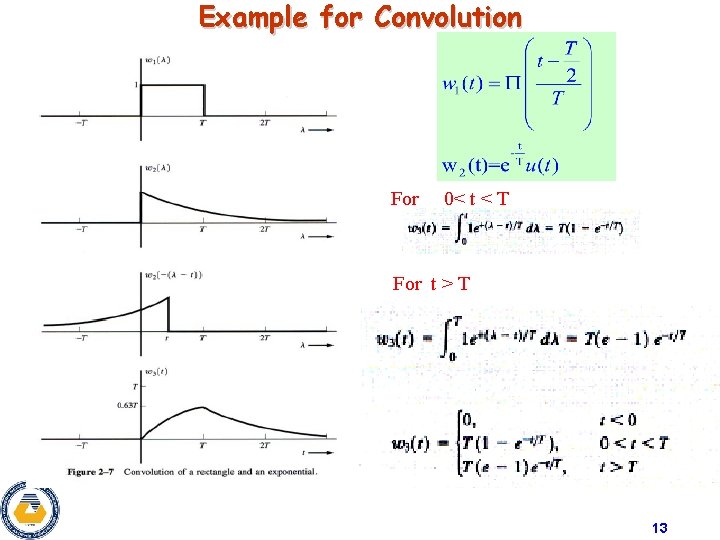
Example for Convolution For 0< t < T For t > T 13

Convolution Ø y(t)=x(t)*z(t)= x(τ)z(t- τ )d τ • Flip one signal and drag it across the other • Area under product at drag offset t is y(t). x(t) -1 0 1 x(t) t t -6 -1 -4 -4 -2 -2 t t 1 -1 2 0 t-1 z(2 -t) z(0 -t) -1 z(t-t) z(t) 0 z(-2 -t) z(-6 -t) -6 z(t) 1 t t t+1 z(4 -t) t 2 y(t) 0 1 2 t 14