Algorithms Lecture 26 Quicksort Quicksort Up to now

Algorithms Lecture 26

Quicksort

Quicksort • Up to now, we were (mostly) looking at randomized algorithms that have some fixed running time, but fail with some probability – We were interested in the failure probability • Here we look at a randomized algorithm that always succeeds, but whose running time varies – We are interested in the expected running time

Quicksort • A quick, randomized sorting algorithm • The algorithm has a O(n 2) worst-case running time, but O(n log n) expected running time

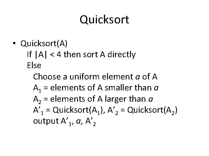
Quicksort • Quicksort(A) If |A| < 4 then sort A directly Else Choose a uniform element a of A A 1 = elements of A smaller than a A 2 = elements of A larger than a A’ 1 = Quicksort(A 1), A’ 2 = Quicksort(A 2) output A’ 1, a, A’ 2

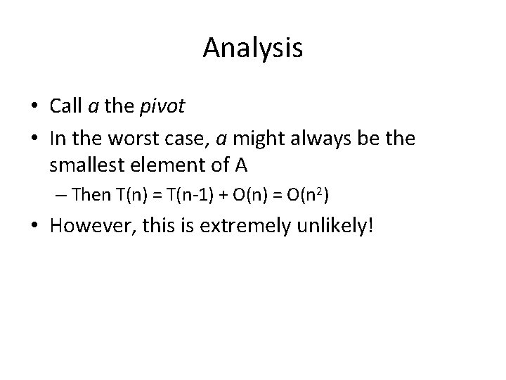
Analysis • Call a the pivot • In the worst case, a might always be the smallest element of A – Then T(n) = T(n-1) + O(n) = O(n 2) • However, this is extremely unlikely!

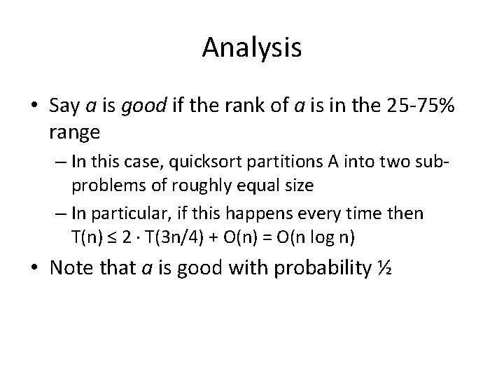
Analysis • Say a is good if the rank of a is in the 25 -75% range – In this case, quicksort partitions A into two subproblems of roughly equal size – In particular, if this happens every time then T(n) ≤ 2 T(3 n/4) + O(n) = O(n log n) • Note that a is good with probability ½

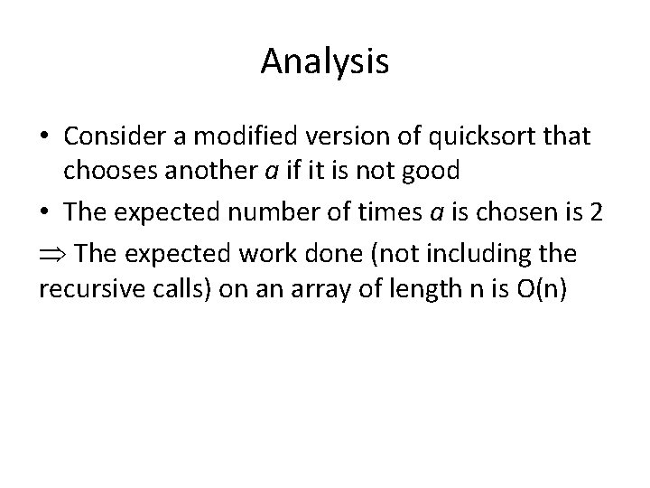
Analysis • Consider a modified version of quicksort that chooses another a if it is not good • The expected number of times a is chosen is 2 The expected work done (not including the recursive calls) on an array of length n is O(n)

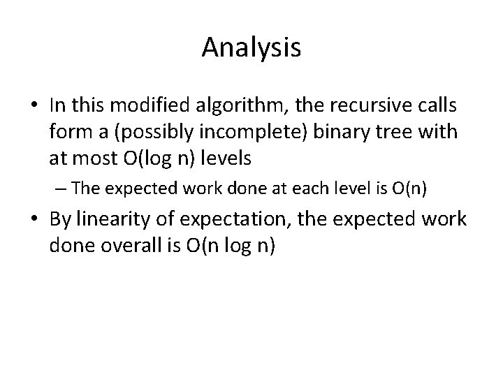
Analysis • In this modified algorithm, the recursive calls form a (possibly incomplete) binary tree with at most O(log n) levels – The expected work done at each level is O(n) • By linearity of expectation, the expected work done overall is O(n log n)

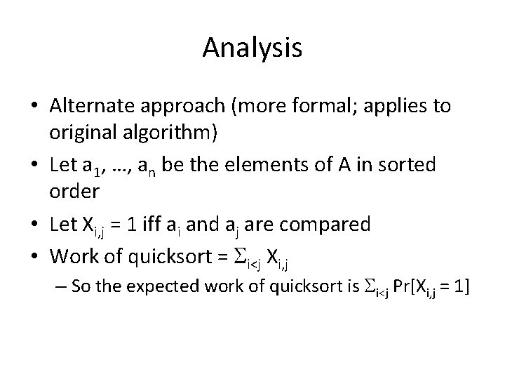
Analysis • Alternate approach (more formal; applies to original algorithm) • Let a 1, …, an be the elements of A in sorted order • Let Xi, j = 1 iff ai and aj are compared • Work of quicksort = i<j Xi, j – So the expected work of quicksort is i<j Pr[Xi, j = 1]

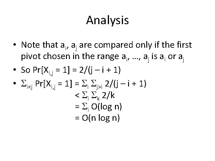
Analysis • Note that ai, aj are compared only if the first pivot chosen in the range ai, …, aj is ai or aj • So Pr[Xi, j = 1] = 2/(j – i + 1) • i<j Pr[Xi, j = 1] = i j>i 2/(j – i + 1) < i k 2/k = i O(log n) = O(n log n)

Analysis • Besides analyzing the expected running time, it is also possible to show that quicksort has good running time with high probability

Hash tables/ load balancing

Hash tables • Want to maintain a set S = {x 1, …, xm} U of size m = |S| using space << |U| – Support the following operations: insert, lookup • Idea: use an array of n linked lists, where an item x S is stored at position H(x) for some hash function H – Insert/lookup involve computing H and traversing a linked list • Want to bound the maximum length of any list

Hash tables • We will model H as a truly random function – Note: this is not correct; it is just a (heuristic) approximation – Can analyze specific hash function families, but this is outside our scope • • A collision is distinct x, x’ with H(x) = H(x’) What is the probability that x and x’ collide? What is the expected number of collisions? What is the expected number of elements that get mapped to position i?

Load balancing • Related problem: map m jobs to n processors by assigning each job to a uniform processor – Note: here the assignments can be truly uniform • Interested in the maximum load on any processor

Analysis • Let Yi be the number of elements mapped to position/processor i • Exp[Yi] = m/n • What is Pr[Yi ≥ c]? • Recall Markov’s inequality: Pr[X ≥ t] ≤ Exp[X]/t • So Pr[Yi ≥ c] ≤ m/cn – Pr[ i : Yi ≥ c] ≤ m/c • This bound is not very useful!

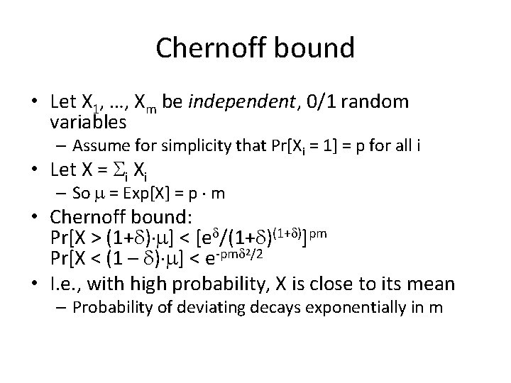
Chernoff bound • Let X 1, …, Xm be independent, 0/1 random variables – Assume for simplicity that Pr[Xi = 1] = p for all i • Let X = i Xi – So = Exp[X] = p m • Chernoff bound: Pr[X > (1+ ) ] < [e /(1+ )]pm 2/2 -pm Pr[X < (1 – ) ] < e • I. e. , with high probability, X is close to its mean – Probability of deviating decays exponentially in m

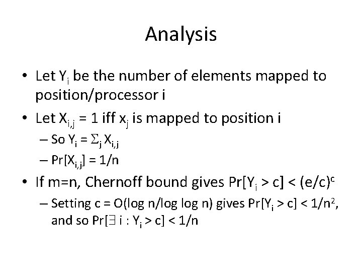
Analysis • Let Yi be the number of elements mapped to position/processor i • Let Xi, j = 1 iff xj is mapped to position i – So Yi = j Xi, j – Pr[Xi, j] = 1/n • If m=n, Chernoff bound gives Pr[Yi > c] < (e/c)c – Setting c = O(log n/log n) gives Pr[Yi > c] < 1/n 2, and so Pr[ i : Yi > c] < 1/n