1 SelfOrganizing Maps Kohonen Networks developed in 1982

. 1 Self-Organizing Maps Kohonen Networks developed in 1982 by Tuevo Kohonen Initially applied to image and sound analysis Represent Self-Organizing Map (SOM) Special class of Neural Networks SOM Convert high-dimensional input to low-dimensional, discrete map Applicable to cluster analysis Structure output nodes to clusters of nodes Nodes in close proximity more similar, compared to those farther apart 2

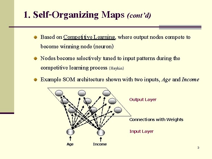
1. Self-Organizing Maps (cont’d) Based on Competitive Learning, where output nodes compete to become winning node (neuron) Nodes become selectively tuned to input patterns during the competitive learning process (Haykin) Example SOM architecture shown with two inputs, Age and Income Output Layer Connections with Weights Input Layer Age Income 3

1. Self-Organizing Maps (cont’d) Every connection between two nodes has weight Weight values initialized randomly 0 – 1 Adjusting weights key feature of learning process Attribute values are normalized or standardized SOMs do not have hidden layer Data passed directly from input layer to output layer 4

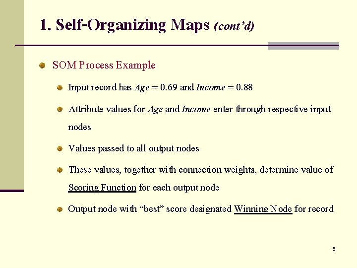
1. Self-Organizing Maps (cont’d) SOM Process Example Input record has Age = 0. 69 and Income = 0. 88 Attribute values for Age and Income enter through respective input nodes Values passed to all output nodes These values, together with connection weights, determine value of Scoring Function for each output node Output node with “best” score designated Winning Node for record 5

1. Self-Organizing Maps (cont’d) SOMs exhibit three characteristics Competition Output nodes compete with one another for “best” score Euclidean Distance function commonly used Winning node produces smallest distance between inputs and connection weights Cooperation Winning node becomes center of neighborhood Output nodes in neighborhood share “excitement” or “reward” 6

1. Self-Organizing Maps (cont’d) Emulates behavior of biological neurons, which are sensitive to output of neighbors Nodes in output layer not directly connected However, share common features because of neighborhood behavior Adaptation Neighborhood nodes participate in adaptation (learning) Weights adjusted to improve score function For subsequent iterations, increases likelihood of winning records with similar values 7

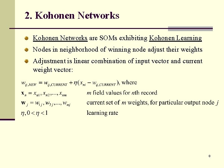
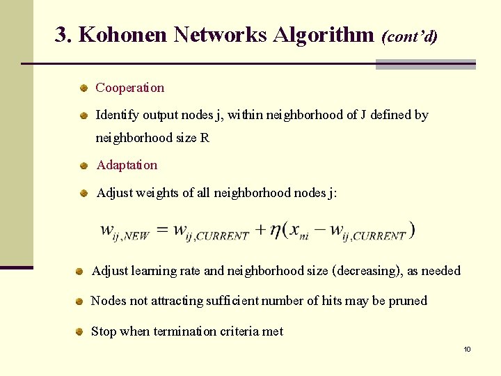
2. Kohonen Networks are SOMs exhibiting Kohonen Learning Nodes in neighborhood of winning node adjust their weights Adjustment is linear combination of input vector and current weight vector: 8

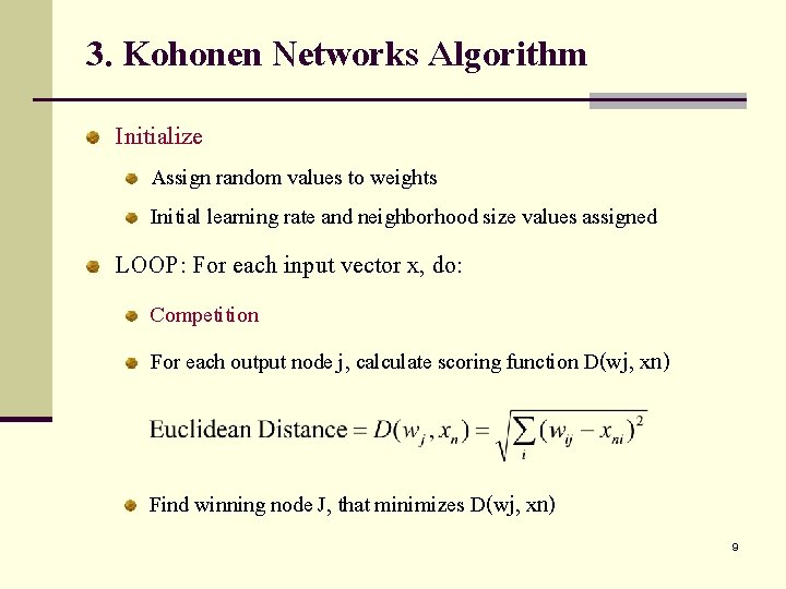
3. Kohonen Networks Algorithm Initialize Assign random values to weights Initial learning rate and neighborhood size values assigned LOOP: For each input vector x, do: Competition For each output node j, calculate scoring function D(wj, xn) Find winning node J, that minimizes D(wj, xn) 9

3. Kohonen Networks Algorithm (cont’d) Cooperation Identify output nodes j, within neighborhood of J defined by neighborhood size R Adaptation Adjust weights of all neighborhood nodes j: Adjust learning rate and neighborhood size (decreasing), as needed Nodes not attracting sufficient number of hits may be pruned Stop when termination criteria met 10

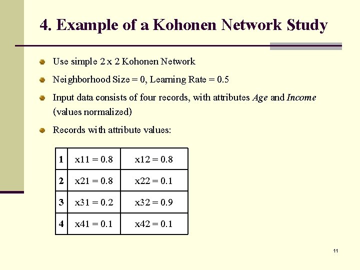
4. Example of a Kohonen Network Study Use simple 2 x 2 Kohonen Network Neighborhood Size = 0, Learning Rate = 0. 5 Input data consists of four records, with attributes Age and Income (values normalized) Records with attribute values: 1 2 3 4 x 11 = 0. 8 x 21 = 0. 8 x 31 = 0. 2 x 41 = 0. 1 x 12 = 0. 8 x 22 = 0. 1 x 32 = 0. 9 x 42 = 0. 1 11

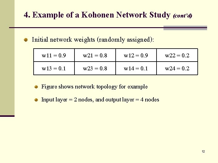
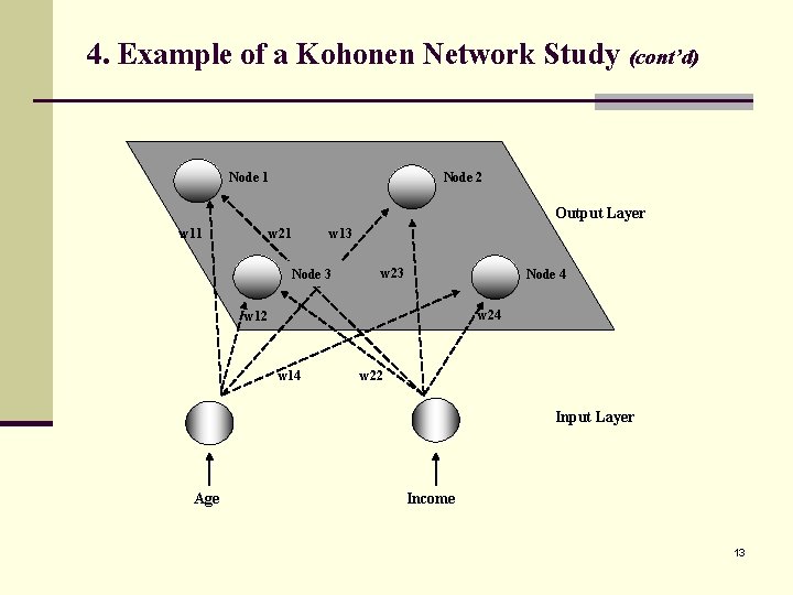
4. Example of a Kohonen Network Study (cont’d) Initial network weights (randomly assigned): w 11 = 0. 9 w 13 = 0. 1 w 21 = 0. 8 w 23 = 0. 8 w 12 = 0. 9 w 14 = 0. 1 w 22 = 0. 2 w 24 = 0. 2 Figure shows network topology for example Input layer = 2 nodes, and output layer = 4 nodes 12

4. Example of a Kohonen Network Study (cont’d) Node 1 Node 2 Output Layer w 11 w 21 w 13 Node 3 w 23 Node 4 w 24 w 12 w 14 w 22 Input Layer Age Income 13

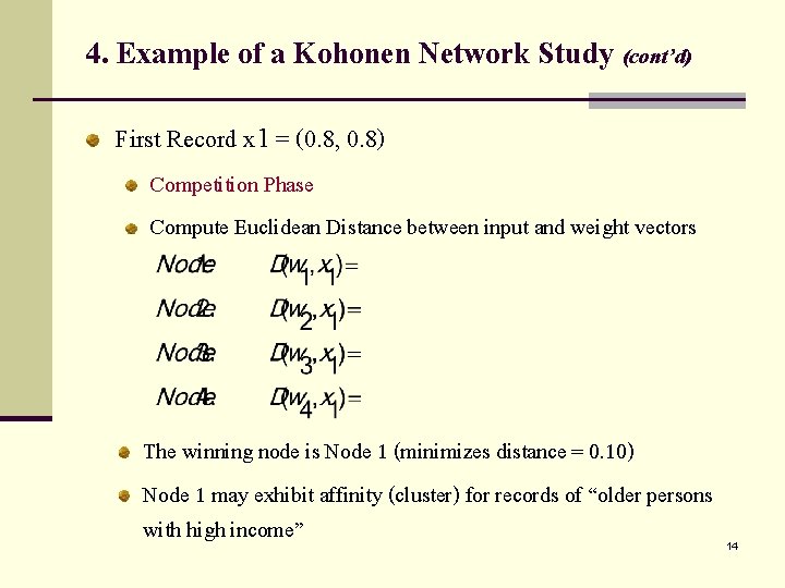
4. Example of a Kohonen Network Study (cont’d) First Record x 1 = (0. 8, 0. 8) Competition Phase Compute Euclidean Distance between input and weight vectors The winning node is Node 1 (minimizes distance = 0. 10) Node 1 may exhibit affinity (cluster) for records of “older persons with high income” 14

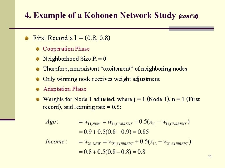
4. Example of a Kohonen Network Study (cont’d) First Record x 1 = (0. 8, 0. 8) Cooperation Phase Neighborhood Size R = 0 Therefore, nonexistent “excitement” of neighboring nodes Only winning node receives weight adjustment Adaptation Phase Weights for Node 1 adjusted, where j = 1 (Node 1), n = 1 (First record), and learning rate = 0. 5: 15

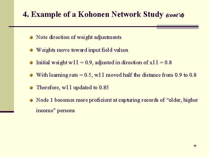
4. Example of a Kohonen Network Study (cont’d) Note direction of weight adjustments Weights move toward input field values Initial weight w 11 = 0. 9, adjusted in direction of x 11 = 0. 8 With learning rate = 0. 5, w 11 moved half the distance from 0. 9 to 0. 8 Therefore, w 11 updated to 0. 85 Node 1 becomes more proficient at capturing records of “older, higher income” persons 16

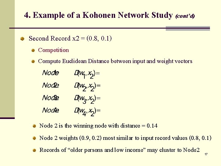
4. Example of a Kohonen Network Study (cont’d) Second Record x 2 = (0. 8, 0. 1) Competition Compute Euclidean Distance between input and weight vectors Node 2 is the winning node with distance = 0. 14 Node 2 weights (0. 9, 0. 2) most similar to input record values (0. 8, 0. 1) Records of “older persons and low income” may cluster to Node 2 17

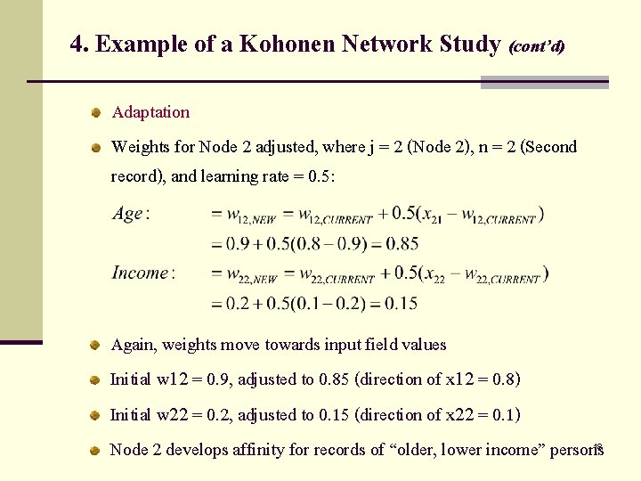
4. Example of a Kohonen Network Study (cont’d) Adaptation Weights for Node 2 adjusted, where j = 2 (Node 2), n = 2 (Second record), and learning rate = 0. 5: Again, weights move towards input field values Initial w 12 = 0. 9, adjusted to 0. 85 (direction of x 12 = 0. 8) Initial w 22 = 0. 2, adjusted to 0. 15 (direction of x 22 = 0. 1) Node 2 develops affinity for records of “older, lower income” persons 18

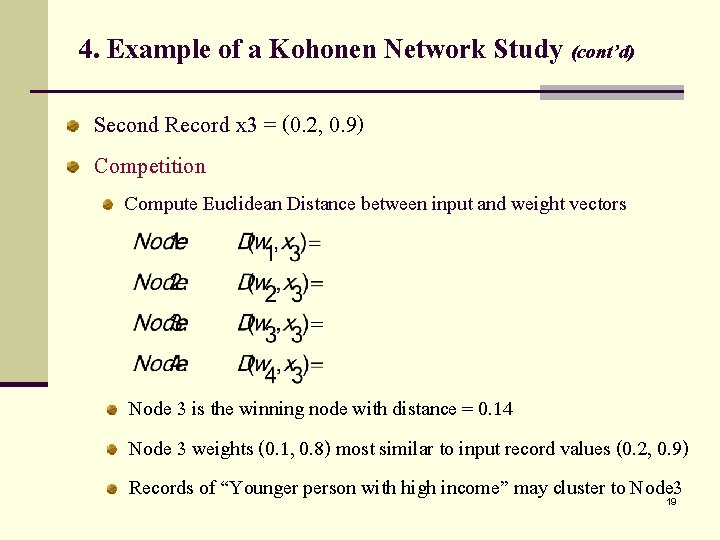
4. Example of a Kohonen Network Study (cont’d) Second Record x 3 = (0. 2, 0. 9) Competition Compute Euclidean Distance between input and weight vectors Node 3 is the winning node with distance = 0. 14 Node 3 weights (0. 1, 0. 8) most similar to input record values (0. 2, 0. 9) Records of “Younger person with high income” may cluster to Node 3 19

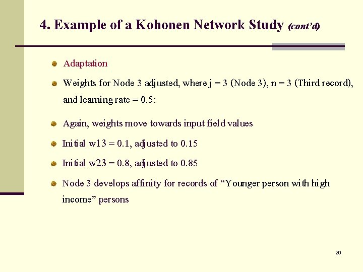
4. Example of a Kohonen Network Study (cont’d) Adaptation Weights for Node 3 adjusted, where j = 3 (Node 3), n = 3 (Third record), and learning rate = 0. 5: Again, weights move towards input field values Initial w 13 = 0. 1, adjusted to 0. 15 Initial w 23 = 0. 8, adjusted to 0. 85 Node 3 develops affinity for records of “Younger person with high income” persons 20

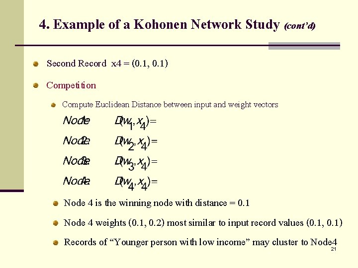
4. Example of a Kohonen Network Study (cont’d) Second Record x 4 = (0. 1, 0. 1) Competition Compute Euclidean Distance between input and weight vectors Node 4 is the winning node with distance = 0. 1 Node 4 weights (0. 1, 0. 2) most similar to input record values (0. 1, 0. 1) Records of “Younger person with low income” may cluster to Node 4 21

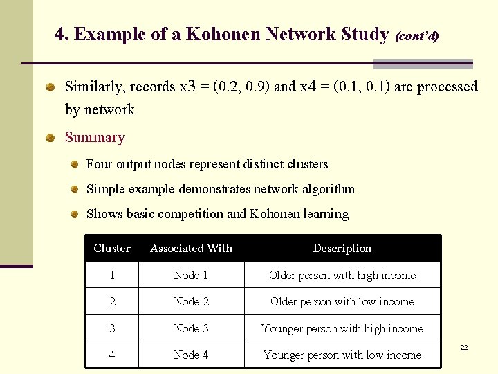
4. Example of a Kohonen Network Study (cont’d) Similarly, records x 3 = (0. 2, 0. 9) and x 4 = (0. 1, 0. 1) are processed by network Summary Four output nodes represent distinct clusters Simple example demonstrates network algorithm Shows basic competition and Kohonen learning Cluster 1 2 3 4 Associated With Node 1 Node 2 Node 3 Node 4 Description Older person with high income Older person with low income Younger person with high income Younger person with low income 22