1 CSCI 104 Splay Trees Mark Redekopp Aaron

1 CSCI 104 Splay Trees Mark Redekopp Aaron Cote’

2 Splay Tree Intro • Another map/set implementation (storing keys or key/value pairs) – Insert, Remove, Find • Recall…To do m inserts/finds/removes on an AVLTree w/ n elements would cost? – O(m*log(n)) • Splay trees have a worst case find, insert, delete time of… – O(n) • However, they guarantee that if you do m operations on a splay tree with n elements that the total time is – O(m*log(n)) [i. e. this is something called amortized analysis] • They have a further benefit that recently accessed elements will be near the top of the tree – In fact, the most recently accessed item is always at the top of the tree

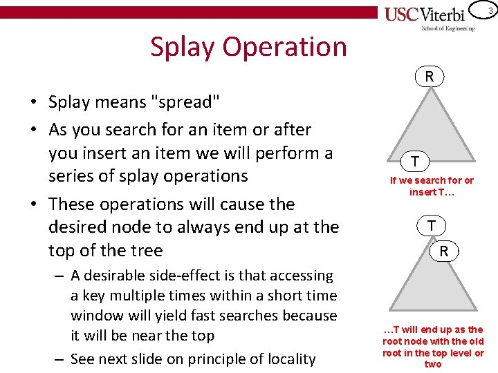
3 Splay Operation R • Splay means "spread" • As you search for an item or after you insert an item we will perform a series of splay operations • These operations will cause the desired node to always end up at the top of the tree – A desirable side-effect is that accessing a key multiple times within a short time window will yield fast searches because it will be near the top – See next slide on principle of locality T If we search for or insert T… T R …T will end up as the root node with the old root in the top level or two

4 Principle of Locality • 2 dimensions of this principle: space & time • Spatial Locality – Future accesses will likely cluster near current accesses – Instructions and data arrays are sequential (they are all one after the next) • Temporal Locality – Future accesses will likely be to recently accessed items – Same code and data are repeatedly accessed (loops, subroutines, if(x > y) x++; – 90/10 rule: Analysis shows that usually 10% of the written instructions account for 90% of the executed instructions • Splay trees help exploit temporal locality by guaranteeing recently accessed items near the top of the tree

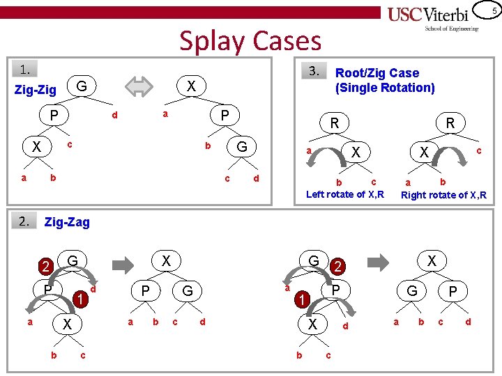
5 Splay Cases 1. G Zig-Zig 3. X P P a d c X a b 2. R G b c Root/Zig Case (Single Rotation) R X a d X c b Left rotate of X, R c b a Right rotate of X, R Zig-Zag G 2 P X 1 b P a X a d c G a G b c P 1 d X b X 2 G d c a P b c d

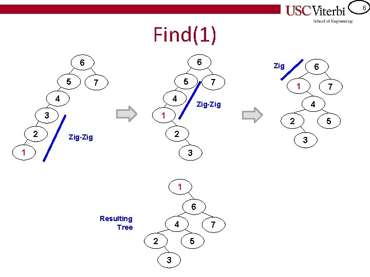
6 Find(1) 6 6 5 5 7 2 1 7 4 Zig-Zig 1 3 6 7 4 4 Zig 2 2 Zig-Zig 1 3 3 1 6 Resulting Tree 4 2 7 5 3 5

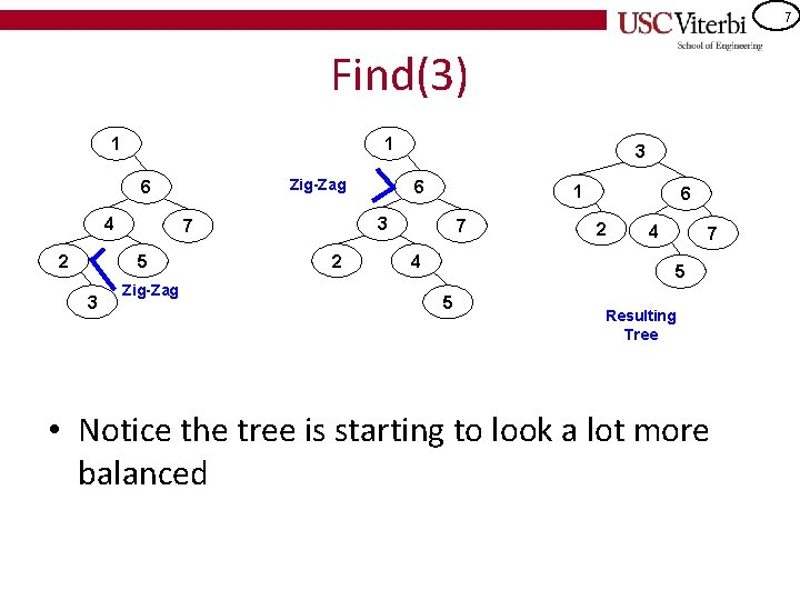
7 Find(3) 1 1 Zig-Zag 6 4 2 3 Zig-Zag 6 1 3 7 5 3 2 7 4 6 2 4 7 5 5 Resulting Tree • Notice the tree is starting to look a lot more balanced

8 Worst Case • Suppose you want to make the average runtime look bad, you might try to always access the _______ node in the tree – Deepest • But splay trees have a property that as we keep accessing deep nodes the tree starts to balance and thus access to deep nodes start by costing O(n) but soon start costing O(log n)

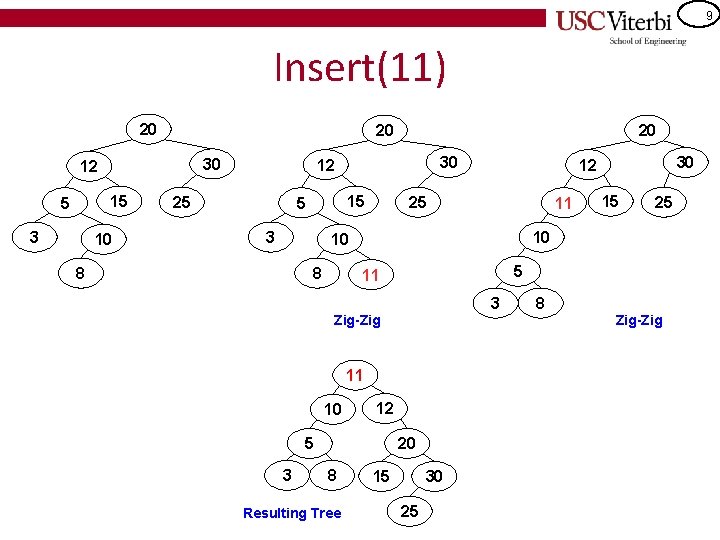
9 Insert(11) 20 20 30 12 15 5 3 10 20 30 12 25 15 5 3 25 11 8 3 Zig-Zig 11 12 5 3 20 8 Resulting Tree 25 5 11 10 15 10 10 8 30 12 15 30 25 8 Zig-Zig

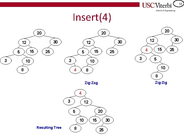
10 Insert(4) 20 30 12 15 5 3 20 20 25 15 5 3 10 8 4 15 4 25 3 10 30 12 5 10 8 8 Zig-Zig Zig-Zag 4 3 12 20 5 10 Resulting Tree 8 15 30 25 25

11 Activity • Go to – https: //www. cs. usfca. edu/~galles/visualization/Splay. Tree. html – Try to be an adversary by inserting and finding elements that would cause O(n) each time

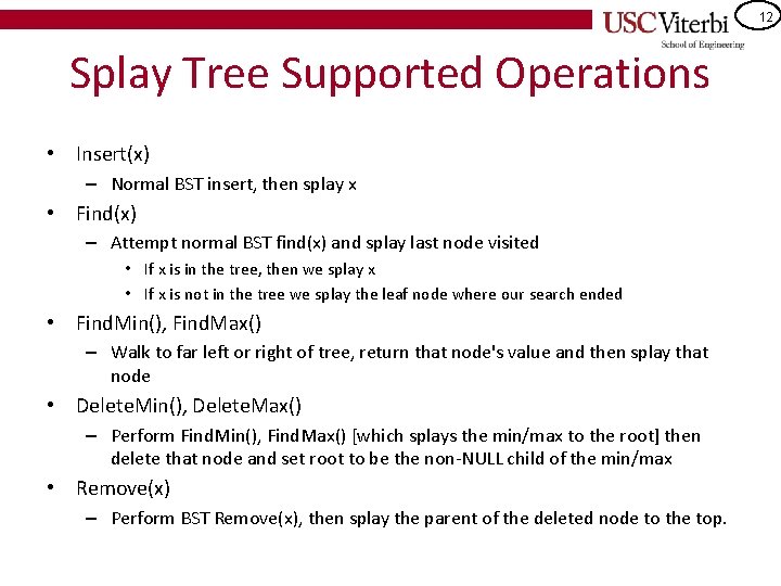
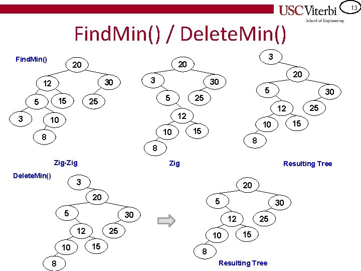
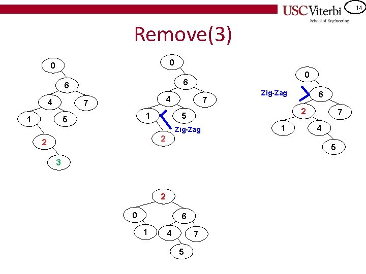
12 Splay Tree Supported Operations • Insert(x) – Normal BST insert, then splay x • Find(x) – Attempt normal BST find(x) and splay last node visited • If x is in the tree, then we splay x • If x is not in the tree we splay the leaf node where our search ended • Find. Min(), Find. Max() – Walk to far left or right of tree, return that node's value and then splay that node • Delete. Min(), Delete. Max() – Perform Find. Min(), Find. Max() [which splays the min/max to the root] then delete that node and set root to be the non-NULL child of the min/max • Remove(x) – Perform BST Remove(x), then splay the parent of the deleted node to the top.

13 Find. Min() / Delete. Min() Find. Min() 20 20 15 3 3 30 12 5 3 30 5 25 20 5 25 10 8 Delete. Min() 15 8 Zig Resulting Tree 3 20 20 5 5 30 8 15 30 25 12 10 15 10 8 Zig-Zig 25 12 12 10 30 10 15 8 Resulting Tree

14 Remove(3) 0 0 6 4 4 7 1 0 6 1 5 7 2 1 7 4 5 3 2 0 6 1 6 2 5 Zig-Zag 2 Zig-Zag 4 7 5

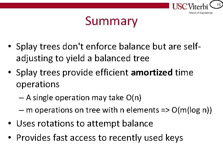
15 Summary • Splay trees don't enforce balance but are selfadjusting to yield a balanced tree • Splay trees provide efficient amortized time operations – A single operation may take O(n) – m operations on tree with n elements => O(m(log n)) • Uses rotations to attempt balance • Provides fast access to recently used keys