1 3 d Deconvolve Advanced Features Et cetera

– 1– 3 d. Deconvolve Advanced Features Et cetera Just in case you weren’t confused enough already

– 9– IM Regression - 1 • IM = Individual Modulation H Compute separate amplitude of response for each stimulus o Instead of computing average amplitude of responses to multiple stimuli in the same class H Response amplitudes ( s) for each individual block/event will be highly noisy o Can’t use individual activation map for much o Must pool the computed s in some further statistical analysis (t-test via 3 dttest? inter-voxel correlations in the s? correlate s with something else? ) H Usage: -stim_times_IM k tname model o Like -stim_times, but creates a separate regression matrix column for each time given

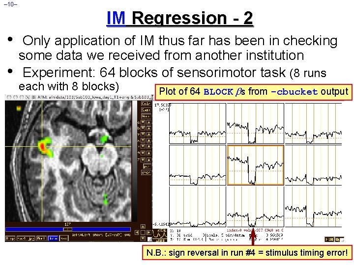
– 10– IM Regression - 2 • • Only application of IM thus far has been in checking some data we received from another institution Experiment: 64 blocks of sensorimotor task (8 runs each with 8 blocks) Plot of 64 BLOCK s from -cbucket output N. B. : sign reversal in run #4 = stimulus timing error!

– 11– IM Regression - 3 • • IM works naturally with blocks, which only have 1 amplitude parameter per stimulus With event-related experiment and deconvolution, have multiple amplitude parameters per stimulus H Difficulty: each event in same class won’t get the same shaped HRF this way H Desideratum: allow response shape to vary (that’s deconvolution), but only allow amplitude to vary between responses in the same stimulus class H Problem: get unknowns that multiply each other (shape parameters amplitude parameters) — and we step outside the realm of linear analysis H Possible solution: semi-linear regression (nonlinear in global shape parameters, linear in local amplitude params)

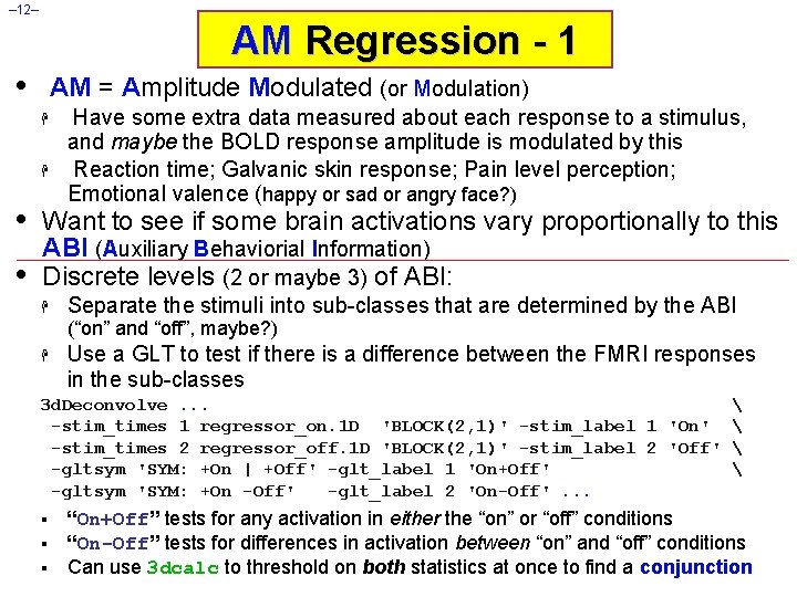
– 12– AM Regression - 1 • AM = Amplitude Modulated (or Modulation) H H • • Have some extra data measured about each response to a stimulus, and maybe the BOLD response amplitude is modulated by this Reaction time; Galvanic skin response; Pain level perception; Emotional valence (happy or sad or angry face? ) Want to see if some brain activations vary proportionally to this ABI (Auxiliary Behaviorial Information) Discrete levels (2 or maybe 3) of ABI: H Separate the stimuli into sub-classes that are determined by the ABI (“on” and “off”, maybe? ) H Use a GLT to test if there is a difference between the FMRI responses in the sub-classes 3 d. Deconvolve. . . -stim_times 1 regressor_on. 1 D 'BLOCK(2, 1)' -stim_label 1 'On' -stim_times 2 regressor_off. 1 D 'BLOCK(2, 1)' -stim_label 2 'Off' -gltsym 'SYM: +On | +Off' -glt_label 1 'On+Off' -gltsym 'SYM: +On -Off' -glt_label 2 'On-Off'. . . § § § “On+Off” tests for any activation in either the “on” or “off” conditions “On-Off” tests for differences in activation between “on” and “off” conditions Can use 3 dcalc to threshold on both statistics at once to find a conjunction

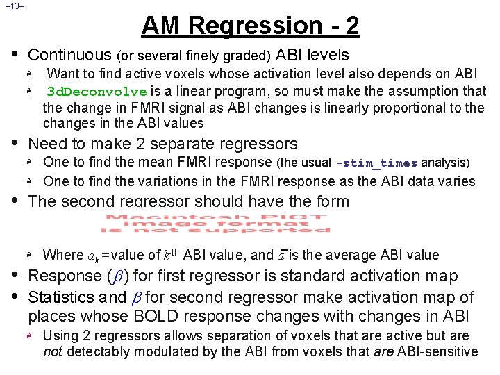
– 13– AM Regression - 2 • Continuous (or several finely graded) ABI levels H H • Need to make 2 separate regressors H • • • Want to find active voxels whose activation level also depends on ABI 3 d. Deconvolve is a linear program, so must make the assumption that the change in FMRI signal as ABI changes is linearly proportional to the changes in the ABI values H One to find the mean FMRI response (the usual -stim_times analysis) One to find the variations in the FMRI response as the ABI data varies The second regressor should have the form H Where ak = value of k th ABI value, and a is the average ABI value Response ( ) for first regressor is standard activation map Statistics and for second regressor make activation map of places whose BOLD response changes with changes in ABI H Using 2 regressors allows separation of voxels that are active but are not detectably modulated by the ABI from voxels that are ABI-sensitive

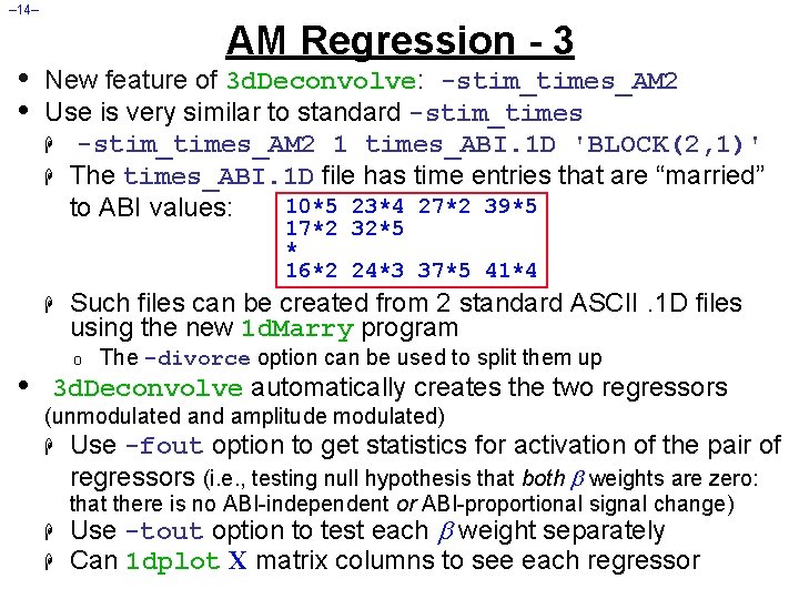
– 14– • • AM Regression - 3 New feature of 3 d. Deconvolve: -stim_times_AM 2 Use is very similar to standard -stim_times H -stim_times_AM 2 1 times_ABI. 1 D 'BLOCK(2, 1)' H The times_ABI. 1 D file has time entries that are “married” 10*5 23*4 27*2 39*5 to ABI values: 17*2 32*5 * 16*2 24*3 37*5 41*4 H • Such files can be created from 2 standard ASCII. 1 D files using the new 1 d. Marry program o The -divorce option can be used to split them up 3 d. Deconvolve automatically creates the two regressors (unmodulated and amplitude modulated) H Use -fout option to get statistics for activation of the pair of regressors (i. e. , testing null hypothesis that both weights are zero: that there is no ABI-independent or ABI-proportional signal change) H H Use -tout option to test each weight separately Can 1 dplot X matrix columns to see each regressor

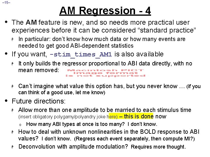
– 15– AM Regression - 4 • The AM feature is new, and so needs more practical user experiences before it can be considered “standard practice” H • • In particular: don’t know how much data or how many events are needed to get good ABI-dependent statistics If you want, -stim_times_AM 1 is also available H It only builds the regressor proportional to ABI data directly, with no mean removed: H Can’t imagine what value this option has, but you never know … (if you can think of a good use, let me know) Future directions: H Allow more than one amplitude to be married to each stimulus time (insert obligatory polygamy/polyandry joke here) – this is done now o H H How many ABI types at once is too many? I don’t know. How to deal with unknown nonlinearities in the BOLD response to ABI values? I don’t know. (Regress each event separately, then compute MI? ) Deconvolution with amplitude modulation? Requires more thought.

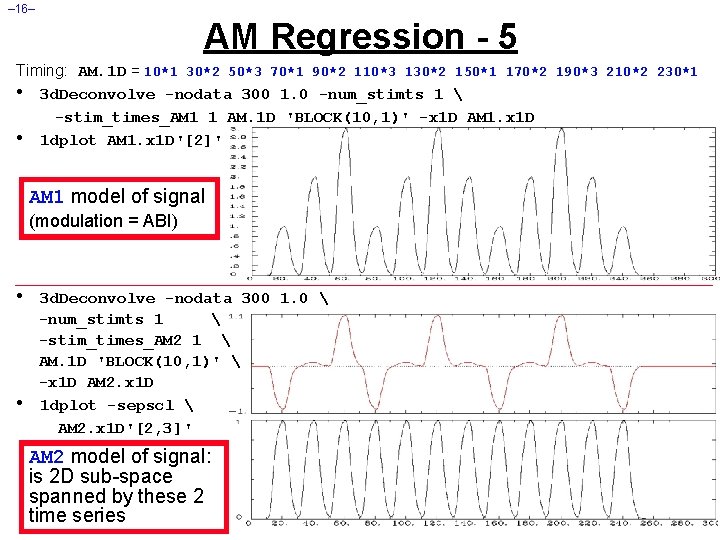
– 16– AM Regression - 5 Timing: AM. 1 D = 10*1 30*2 50*3 70*1 90*2 110*3 130*2 150*1 170*2 190*3 210*2 230*1 • 3 d. Deconvolve -nodata 300 1. 0 -num_stimts 1 -stim_times_AM 1 1 AM. 1 D 'BLOCK(10, 1)' -x 1 D AM 1. x 1 D • 1 dplot AM 1. x 1 D'[2]' AM 1 model of signal (modulation = ABI) • • 3 d. Deconvolve -nodata 300 1. 0 -num_stimts 1 -stim_times_AM 2 1 AM. 1 D 'BLOCK(10, 1)' -x 1 D AM 2. x 1 D 1 dplot -sepscl AM 2. x 1 D'[2, 3]' AM 2 model of signal: is 2 D sub-space spanned by these 2 time series

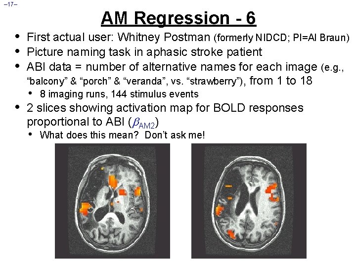
– 17– • • AM Regression - 6 First actual user: Whitney Postman (formerly NIDCD; PI=Al Braun) Picture naming task in aphasic stroke patient ABI data = number of alternative names for each image (e. g. , “balcony” & “porch” & “veranda”, vs. “strawberry”), from 1 to 18 • 8 imaging runs, 144 stimulus events 2 slices showing activation map for BOLD responses proportional to ABI ( AM 2) • What does this mean? Don’t ask me!

– 18– AM Regression - 7 • • • Alternative: use IM to get individual s for each block/event and then do external regression statistics on those values Could do nonlinear fitting (to these s) via 3 d. NLfim, or inter-class contrasts via 3 dttest, 3 d. LME, 3 d. ANOVA, or intra-class correlations via 3 d. ICC, etc. What is better: AM or IM+something more ? • We don’t know – experience with these options is limited thus far – you can always try both! • If AM doesn’t fit your models/ideas, then IM+ is clearly the way to go • Probably need to consult with SSCC to get some hints/advice

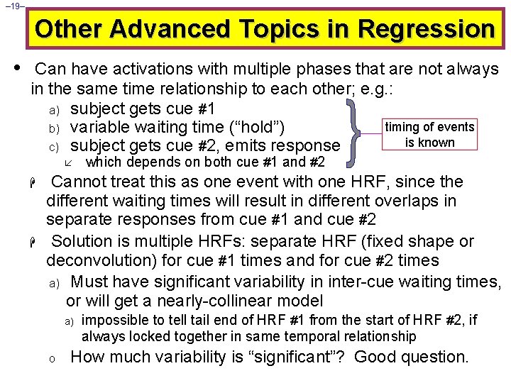
– 19– Other Advanced Topics in Regression • Can have activations with multiple phases that are not always in the same time relationship to each other; e. g. : a) subject gets cue #1 timing of events b) variable waiting time (“hold”) is known c) subject gets cue #2, emits response å H H which depends on both cue #1 and #2 Cannot treat this as one event with one HRF, since the different waiting times will result in different overlaps in separate responses from cue #1 and cue #2 Solution is multiple HRFs: separate HRF (fixed shape or deconvolution) for cue #1 times and for cue #2 times a) Must have significant variability in inter-cue waiting times, or will get a nearly-collinear model a) o impossible to tell tail end of HRF #1 from the start of HRF #2, if always locked together in same temporal relationship How much variability is “significant”? Good question.

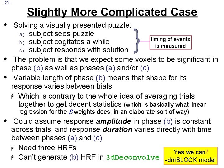
– 20– Slightly More Complicated Case • • Solving a visually presented puzzle: a) subject sees puzzle timing of events b) subject cogitates a while is measured c) subject responds with solution The problem is that we expect some voxels to be significant in phase (b) as well as phases (a) and/or (c) Variable length of phase (b) means that shape for its response varies between trials H Which is contrary to the whole idea of averaging trials together to get decent statistics (which is basically what linear regression for the weights does, in an elaborate sort of way) Could assume response amplitude in phase (b) is constant across trials, and response duration varies directly with time between phases (a) and (c) H Need three HRFs Yes we can! H Can’t generate (b) HRF in 3 d. Deconvolve -dm. BLOCK model

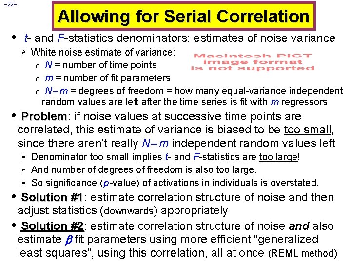
– 22– • Allowing for Serial Correlation t- and F-statistics denominators: estimates of noise variance H White noise estimate of variance: o N = number of time points o m = number of fit parameters o N – m = degrees of freedom = how many equal-variance independent random values are left after the time series is fit with m regressors • Problem: Problem if noise values at successive time points are correlated, this estimate of variance is biased to be too small, since there aren’t really N – m independent random values left H H H Denominator too small implies t- and F-statistics are too large! And number of degrees of freedom is also too large. So significance (p -value) of activations in individuals is overstated. • Solution #1: #1 estimate correlation structure of noise and then adjust statistics (downwards) appropriately • Solution #2: #2 estimate correlation structure of noise and also estimate fit parameters using more efficient “generalized least squares”, using this correlation, all at once (REML method)

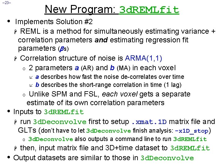
– 23– • New Program: 3 d. REMLfit Implements Solution #2 H REML is a method for simultaneously estimating variance + correlation parameters and estimating regression fit parameters ( s) H Correlation structure of noise is ARMA(1, 1) o 2 parameters a (AR) and b (MA) in each voxel å å a describes how fast the noise de-correlates over time b describes the short-range correlation in time (1 lag) Unlike SPM and FSL, each voxel gets a separate estimate of its own correlation parameters Inputs to 3 d. REMLfit H run 3 d. Deconvolve first to setup. xmat. 1 D matrix file and GLTs (don’t have to let 3 d. Deconvolve finish analysis: -x 1 D_stop) o • 3 d. Deconvolve also outputs a command line to run 3 d. REMLfit then, input matrix file and 3 D+time dataset to 3 d. REMLfit Output datasets are similar to those in 3 d. Deconvolve H

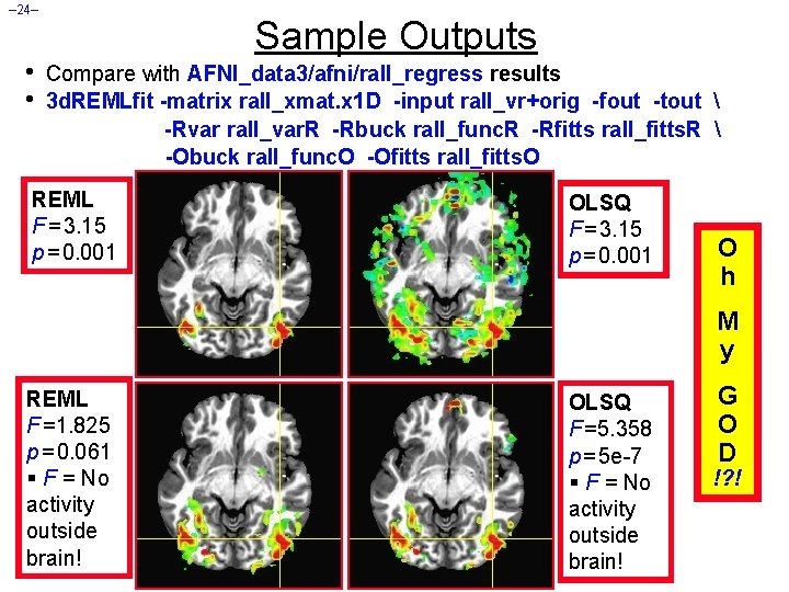
– 24– • • Sample Outputs Compare with AFNI_data 3/afni/rall_regress results 3 d. REMLfit -matrix rall_xmat. x 1 D -input rall_vr+orig -fout -tout -Rvar rall_var. R -Rbuck rall_func. R -Rfitts rall_fitts. R -Obuck rall_func. O -Ofitts rall_fitts. O REML F = 3. 15 p = 0. 001 OLSQ F = 3. 15 p = 0. 001 O h M y REML F =1. 825 p = 0. 061 § F = No activity outside brain! OLSQ F =5. 358 p = 5 e-7 § F = No activity outside brain! G O D !? !

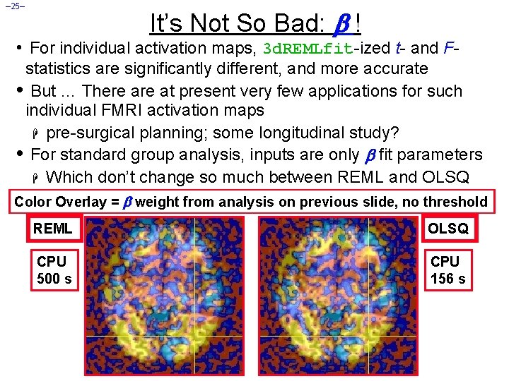
– 25– It’s Not So Bad: ! • For individual activation maps, 3 d. REMLfit-ized t- and Fstatistics are significantly different, and more accurate • But … There at present very few applications for such individual FMRI activation maps H pre-surgical planning; some longitudinal study? • For standard group analysis, inputs are only fit parameters H Which don’t change so much between REML and OLSQ Color Overlay = weight from analysis on previous slide, no threshold REML OLSQ CPU 500 s CPU 156 s

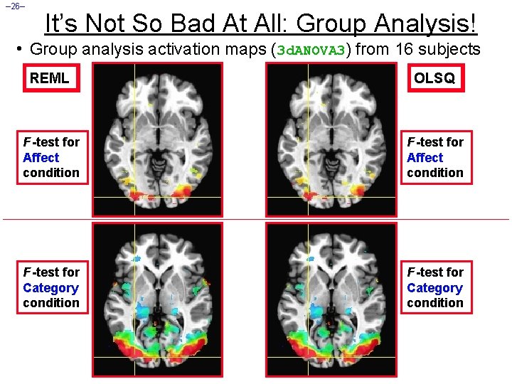
– 26– It’s Not So Bad At All: Group Analysis! • Group analysis activation maps (3 d. ANOVA 3) from 16 subjects REML OLSQ F -test for Affect condition F -test for Category condition

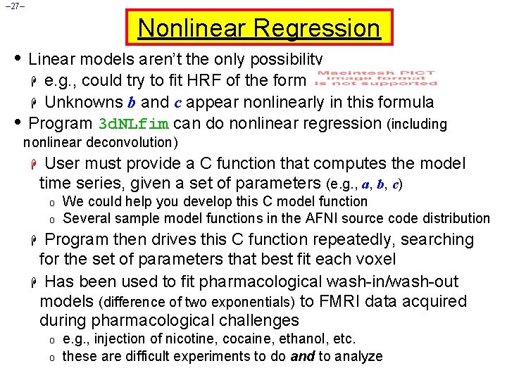
– 27– Nonlinear Regression • Linear models aren’t the only possibility e. g. , could try to fit HRF of the form H Unknowns b and c appear nonlinearly in this formula Program 3 d. NLfim can do nonlinear regression (including H • nonlinear deconvolution) H User must provide a C function that computes the model time series, given a set of parameters (e. g. , a, b, c) o o We could help you develop this C model function Several sample model functions in the AFNI source code distribution Program then drives this C function repeatedly, searching for the set of parameters that best fit each voxel H Has been used to fit pharmacological wash-in/wash-out models (difference of two exponentials) to FMRI data acquired during pharmacological challenges H o o e. g. , injection of nicotine, cocaine, ethanol, etc. these are difficult experiments to do and to analyze

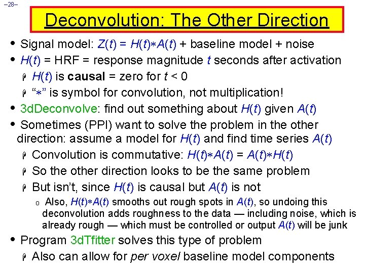
– 28– Deconvolution: The Other Direction • Signal model: Z(t) = H(t) A(t) + baseline model + noise • H(t) = HRF = response magnitude t seconds after activation H(t) is causal = zero for t < 0 H “ ” is symbol for convolution, not multiplication! • 3 d. Deconvolve: find out something about H(t) given A(t) • Sometimes (PPI) want to solve the problem in the other direction: assume a model for H(t) and find time series A(t) H Convolution is commutative: H(t) A(t) = A(t) H So the other direction looks to be the same problem H But isn’t, since H(t) is causal but A(t) is not H o Also, H(t) A(t) smooths out rough spots in A(t), so undoing this deconvolution adds roughness to the data — including noise, which is already rough — which must be controlled or output A(t) will be junk • Program 3 d. Tfitter solves this type of problem H Also can allow for per voxel baseline model components