Using Simulation to Enhance Statistical Understanding Michael Sullivan

Using Simulation to Enhance Statistical Understanding Michael Sullivan Joliet Junior College sullystats@gmail. com msulliva@jjc. edu www. sullystats. com

Randomness • The word random suggests an unpredictable result or outcome. • Three types of randomness are presented in Introductory Statistics • Random selection • Random assignment • Random process

Random Selection • https: //data. cityofchicago. org/ • Go to Administration & Finance • Download the Salary Report • File Contains Salaried and Hourly Employees • • • Extract only the salaried employees Find the population mean salary Have each of your students find a simple random sample of n = 12 employees. What is the sample mean? Great discussion ensues regarding the fact that students are getting different results. Find a second simple random sample of n = 12 employees. What is the sample mean? Find 2000 SRS of size n = 12 and compute the sample mean of each. Draw a histogram.

Stat. Crunch 1. Open the data “Chicago. Salaries” in Stat. Crunch (join the Sully. Stats group). 2. Data > Sample Select “Annual Salary” Enter 12 for Sample Size. Enter number of samples desired. If taking multiple samples, select the “Stacked with sample id” radio button. Decide on a dynamic or fixed seed. Check the box “Open in new data table”. Click Compute! 3. Stat > Summary Stats > Columns Select Sample(variable name). Group by” Sample. Choose the statistic you wish to compute (such as Mean). Check the box “Store in data table. ” Click Compute! Note: Stat. Crunch may say “Whoa! Lots of data…” Click Cancel (do not bin the data). 4. Draw histograms of the sample means to show the variability. Note: To illustrate the properties of the random variable “xbar”, you could do things like find the mean and standard error of xbar and compare to theoretical values.

Example of a Random Process • Red Light

The Law of Large Numbers versus The “Nonexistent” Law of Averages

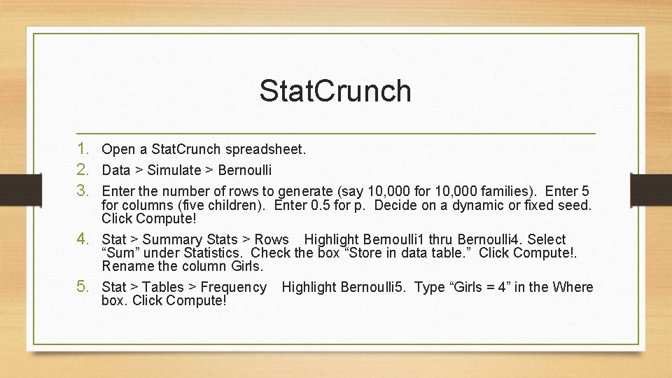
Stat. Crunch 1. Open a Stat. Crunch spreadsheet. 2. Data > Simulate > Bernoulli 3. Enter the number of rows to generate (say 10, 000 for 10, 000 families). Enter 5 for columns (five children). Enter 0. 5 for p. Decide on a dynamic or fixed seed. Click Compute! 4. Stat > Summary Stats > Rows Highlight Bernoulli 1 thru Bernoulli 4. Select “Sum” under Statistics. Check the box “Store in data table. ” Click Compute!. Rename the column Girls. 5. Stat > Tables > Frequency Highlight Bernoulli 5. Type “Girls = 4” in the Where box. Click Compute!

In a random process, the trials are memoryless.

Random Selection • Unplugging refers to eliminating the use of social media, cell phones, and other technology. According to Harris Interactive, the proportion of adult Americans (aged 18 or older) who attempt to “unplug” at least once a week is 0. 45. There approximately 241, 000 adult Americans in the United States. (a) Simulate obtaining a simple random sample of size 500 from the population of adult Americans. How many of the individuals sampled unplug? How many do not unplug? What proportion unplug at least once a week?

Random Selection (b) Simulate obtaining a second simple random sample of size 500 from the population of adult Americans. How many of the individuals sampled unplug? How many do not unplug? What proportion unplug at least once a week? (c) Now simulate obtaining at least 2000 more simple random samples of size 500 from the population. Based on the simulation, what is the probability of obtaining a random sample where the proportion who unplug at least once a week is greater than 0. 50?

Stat. Crunch The Urn Applet 1. Select Applets > Simulation > Urn sampling 2. Decide on the color ball for Type 1 and the number of balls for Type 1; decide on the color ball for Type 2 and the number of balls for Type 2. Under Sampling, determine the number of balls to select. Under Tally type, decide if you want to track the number of Type 1 balls or proportion of Type 1 balls. Click Compute!

Sampling Distribution of the Slope 1. Find the least-squares regression model using the home run data treating speed off bat as the explanatory variable and distance as the response variable. 2. Find 1000 different SRS of size n = 15 for these data. 3. Find the least-squares regression model for each of the 1000 SRS. 4. Graph the distribution of the estimates of the slope. What is the mean of the 1000 different slopes? 5. Notice the slope standard error for each sample. Draw scatter diagrams of those with small standard errors versus large.

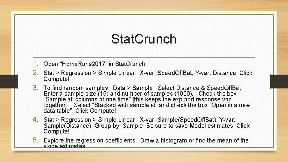
Stat. Crunch 1. Open “Home. Runs 2017” in Stat. Crunch. 2. Stat > Regression > Simple Linear X-var: Speed. Off. Bat; Y-var: Distance Click Compute! 3. To find random samples: Data > Sample Select Distance & Speed. Off. Bat Enter a sample size (15) and number of samples (1000). Check the box “Sample all columns at one time” [this keeps the exp and response var together]. Select “Stacked with sample id” and check the box “Open in a new data table”. Click Compute! 4. Stat > Regression > Simple Linear X-var: Sample(Speed. Off. Bat); Y-var: Sample(Distance) Group by: Sample Be sure to save Model estimates. Click Compute! 5. Explore the regression coefficients. Draw a histogram or find the mean of the slope estimates.

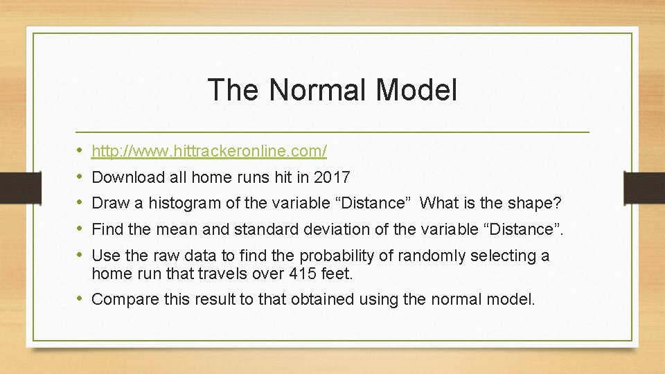
The Normal Model • • • http: //www. hittrackeronline. com/ Download all home runs hit in 2017 Draw a histogram of the variable “Distance” What is the shape? Find the mean and standard deviation of the variable “Distance”. Use the raw data to find the probability of randomly selecting a home run that travels over 415 feet. • Compare this result to that obtained using the normal model.