Statistical Life Expectancy Modelling Pot Life in a

Figure 1 Data description Principal Component Analysis (above) • Good split of the data

Figure 2 Example of confusion between design and process effect Life expectancy increases with

Figure 3 Models and process variables operating ranges Design 1 Life expectancy : •

Figure 4 Start-up date effect or period effect There is a historic and/or a

Slides: 5

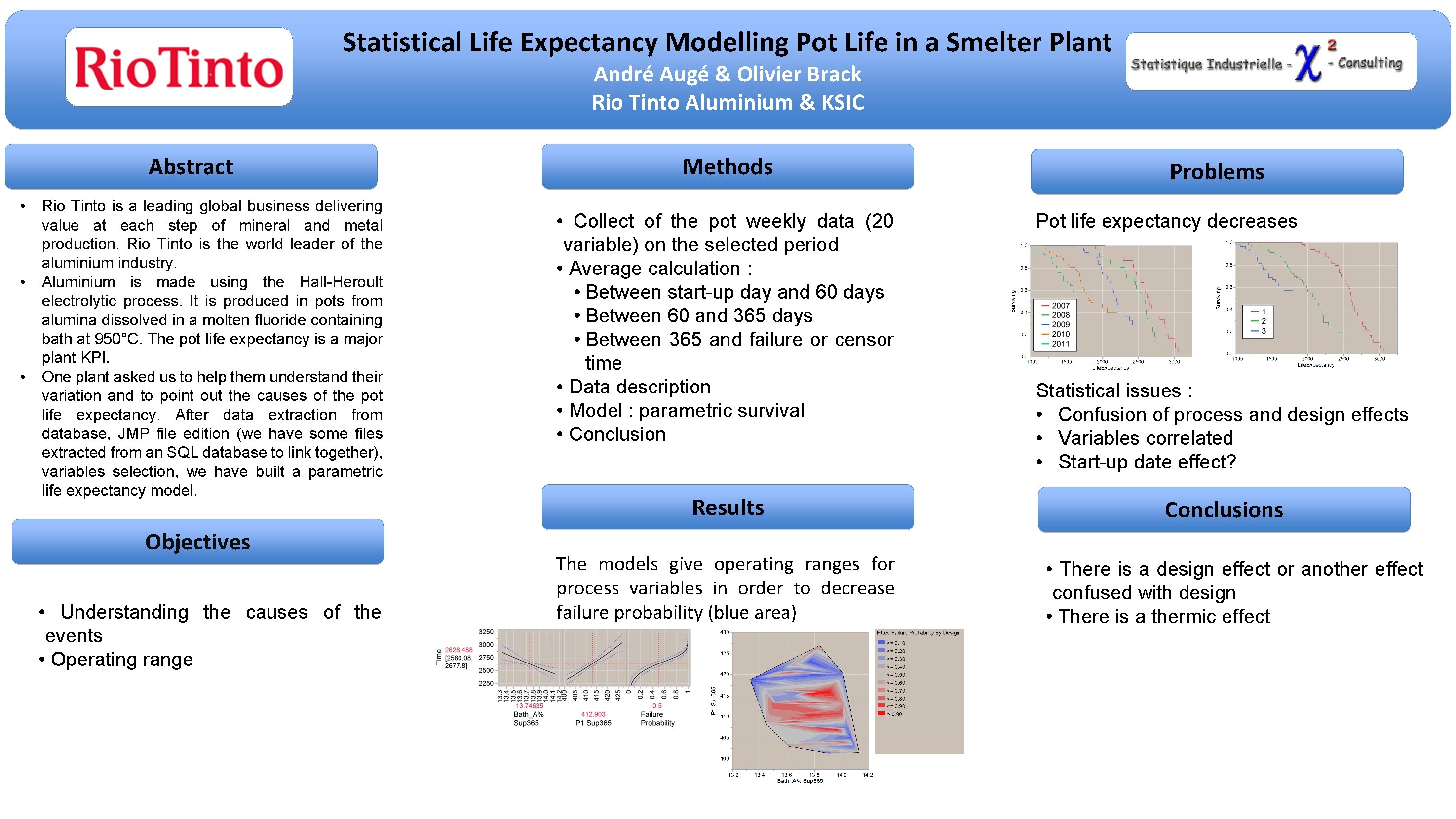
Statistical Life Expectancy Modelling Pot Life in a Smelter Plant André Augé & Olivier Brack Rio Tinto Aluminium & KSIC Abstract • • • Rio Tinto is a leading global business delivering value at each step of mineral and metal production. Rio Tinto is the world leader of the aluminium industry. Aluminium is made using the Hall-Heroult electrolytic process. It is produced in pots from alumina dissolved in a molten fluoride containing bath at 950°C. The pot life expectancy is a major plant KPI. One plant asked us to help them understand their variation and to point out the causes of the pot life expectancy. After data extraction from database, JMP file edition (we have some files extracted from an SQL database to link together), variables selection, we have built a parametric life expectancy model. Objectives • Understanding the causes of the events • Operating range Methods • Collect of the pot weekly data (20 variable) on the selected period • Average calculation : • Between start-up day and 60 days • Between 60 and 365 days • Between 365 and failure or censor time • Data description • Model : parametric survival • Conclusion Results The models give operating ranges for process variables in order to decrease failure probability (blue area) Problems Pot life expectancy decreases Statistical issues : • Confusion of process and design effects • Variables correlated • Start-up date effect? Conclusions • There is a design effect or another effect confused with design • There is a thermic effect

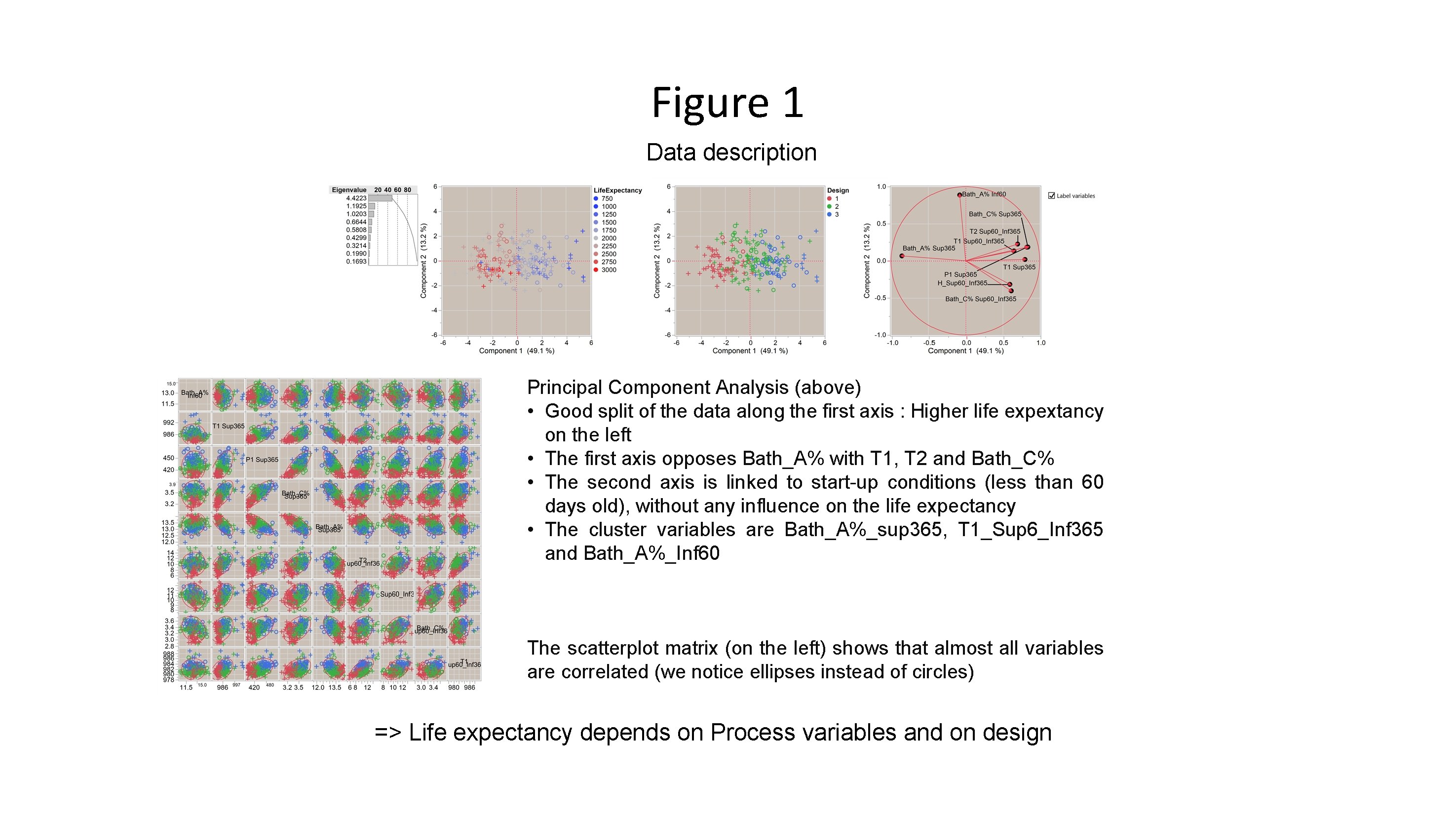
Figure 1 Data description Principal Component Analysis (above) • Good split of the data along the first axis : Higher life expextancy on the left • The first axis opposes Bath_A% with T 1, T 2 and Bath_C% • The second axis is linked to start-up conditions (less than 60 days old), without any influence on the life expectancy • The cluster variables are Bath_A%_sup 365, T 1_Sup 6_Inf 365 and Bath_A%_Inf 60 The scatterplot matrix (on the left) shows that almost all variables are correlated (we notice ellipses instead of circles) => Life expectancy depends on Process variables and on design

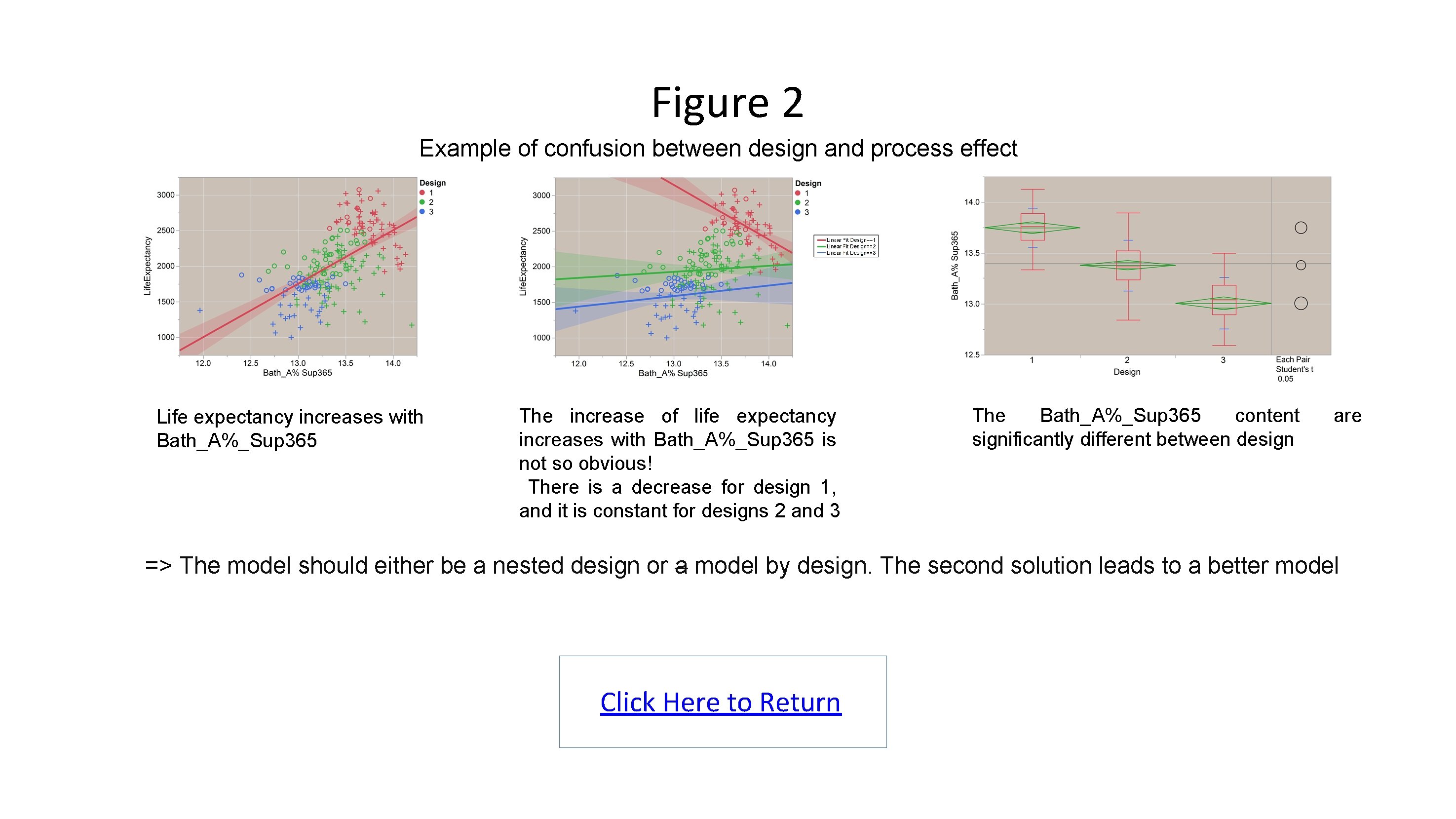
Figure 2 Example of confusion between design and process effect Life expectancy increases with Bath_A%_Sup 365 The increase of life expectancy increases with Bath_A%_Sup 365 is not so obvious! There is a decrease for design 1, and it is constant for designs 2 and 3 The Bath_A%_Sup 365 content significantly different between design are => The model should either be a nested design or a model by design. The second solution leads to a better model Click Here to Return

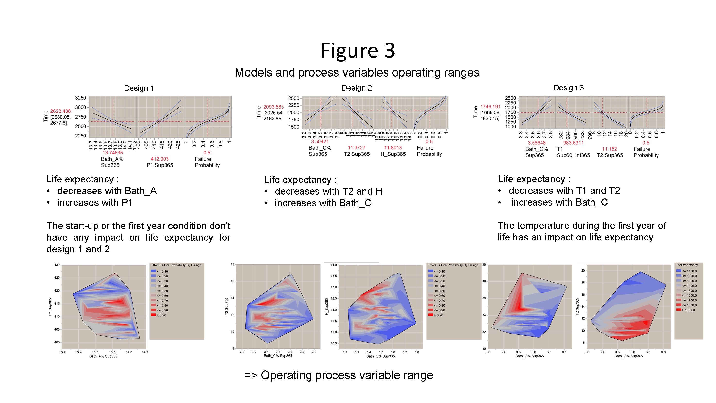
Figure 3 Models and process variables operating ranges Design 1 Life expectancy : • decreases with Bath_A • increases with P 1 Design 2 Life expectancy : • decreases with T 2 and H • increases with Bath_C Design 3 Life expectancy : • decreases with T 1 and T 2 • increases with Bath_C The temperature during the first year of life has an impact on life expectancy The start-up or the first year condition don’t have any impact on life expectancy for design 1 and 2 => Operating process variable range

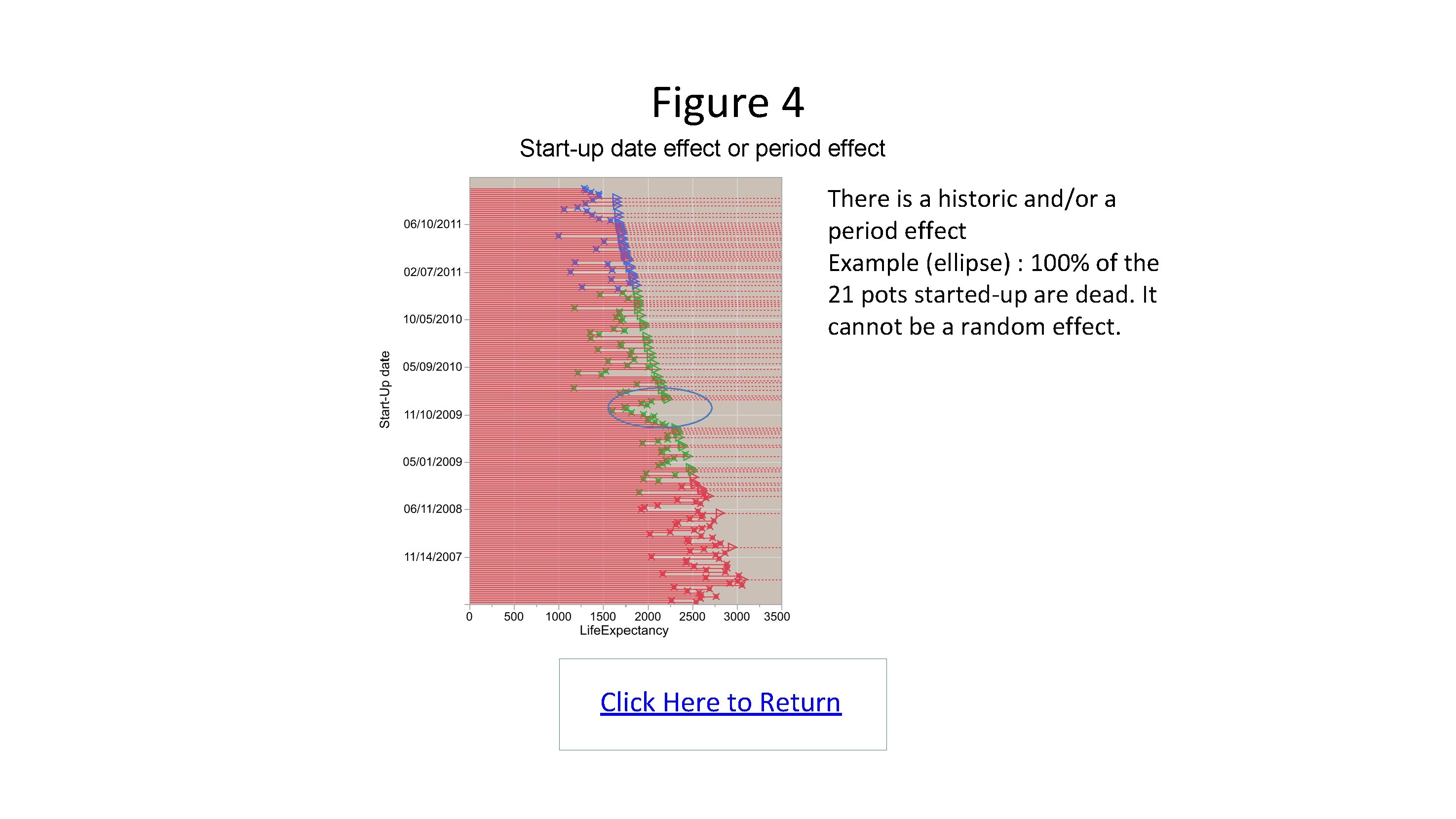
Figure 4 Start-up date effect or period effect There is a historic and/or a period effect Example (ellipse) : 100% of the 21 pots started-up are dead. It cannot be a random effect. Click Here to Return