SPICE Mie mi Dmitry Chirkin UW Madison Updates

SPICE Mie [mi: ] Dmitry Chirkin, UW Madison

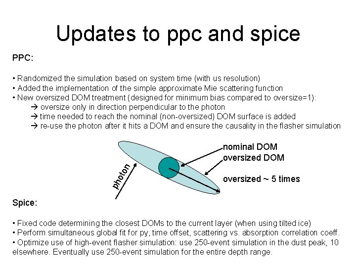
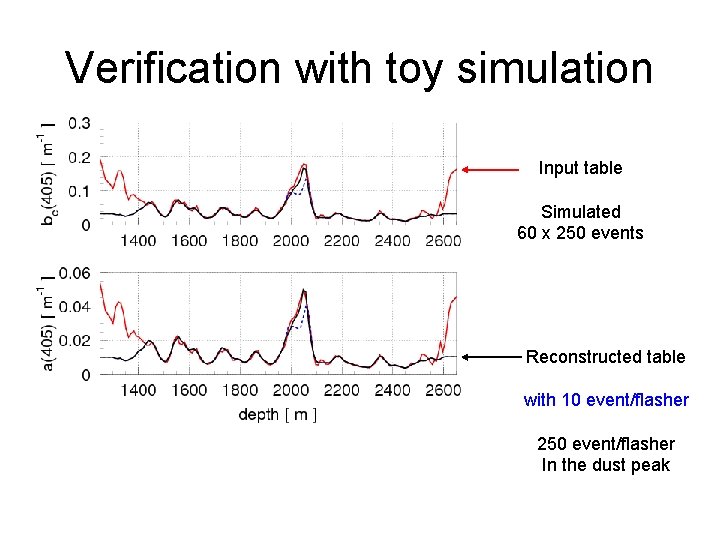
Updates to ppc and spice PPC: • Randomized the simulation based on system time (with us resolution) • Added the implementation of the simple approximate Mie scattering function • New oversized DOM treatment (designed for minimum bias compared to oversize=1): oversize only in direction perpendicular to the photon time needed to reach the nominal (non-oversized) DOM surface is added re-use the photon after it hits a DOM and ensure the causality in the flasher simulation ph oto n nominal DOM oversized ~ 5 times Spice: • Fixed code determining the closest DOMs to the current layer (when using tilted ice) • Perform simultaneous global fit for py, time offset, scattering vs. absorption correlation coeff. • Optimize use of high-event flasher simulation: use 250 -event simulation in the dust peak, 10 elsewhere. Eventually use 250 -event simulation for the entire depth range.

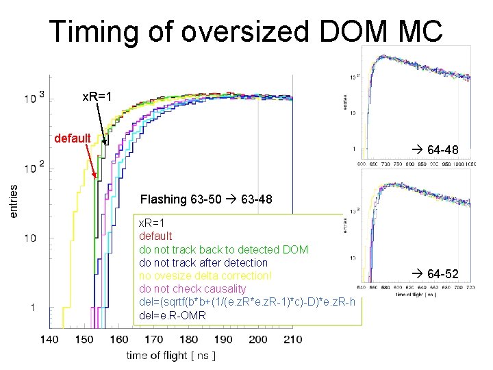
Timing of oversized DOM MC x. R=1 default 64 -48 Flashing 63 -50 63 -48 x. R=1 default do not track back to detected DOM do not track after detection no ovesize delta correction! do not check causality del=(sqrtf(b*b+(1/(e. z. R*e. z. R-1)*c)-D)*e. z. R-h del=e. R-OMR 64 -52

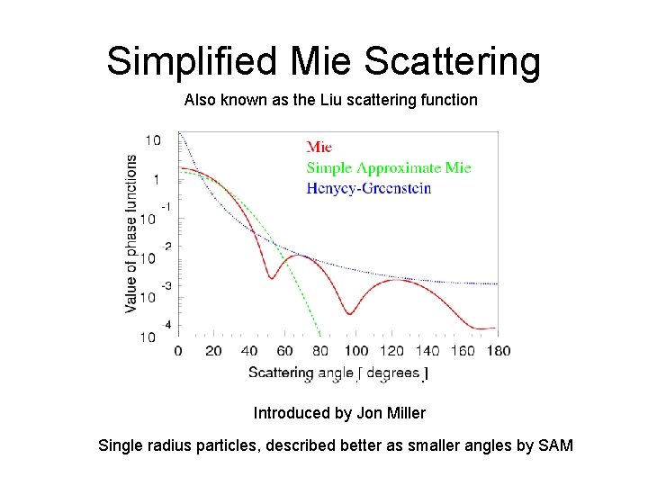
Simplified Mie Scattering Also known as the Liu scattering function Introduced by Jon Miller Single radius particles, described better as smaller angles by SAM

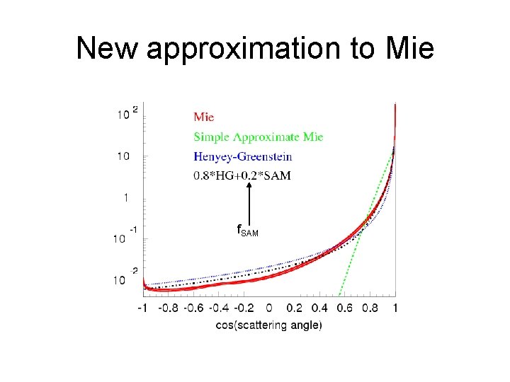
New approximation to Mie f. SAM

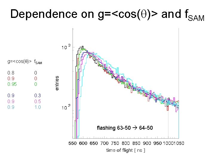
Dependence on g=<cos(q)> and f. SAM g=<cos(q)> f. SAM 0. 8 0. 95 0 0. 9 0. 3 0. 5 1. 0 flashing 63 -50 64 -50

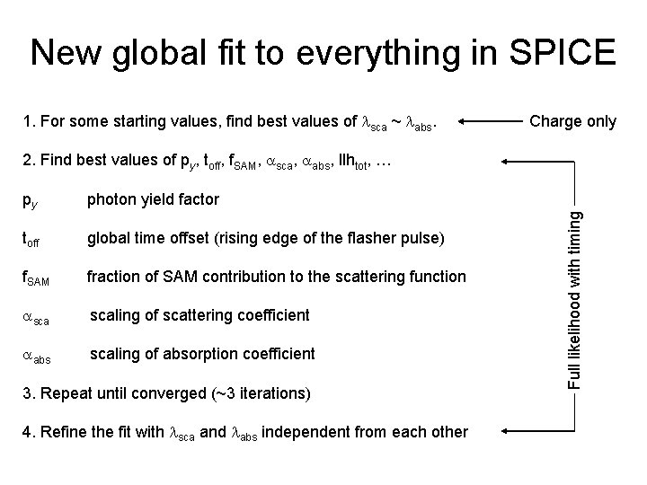
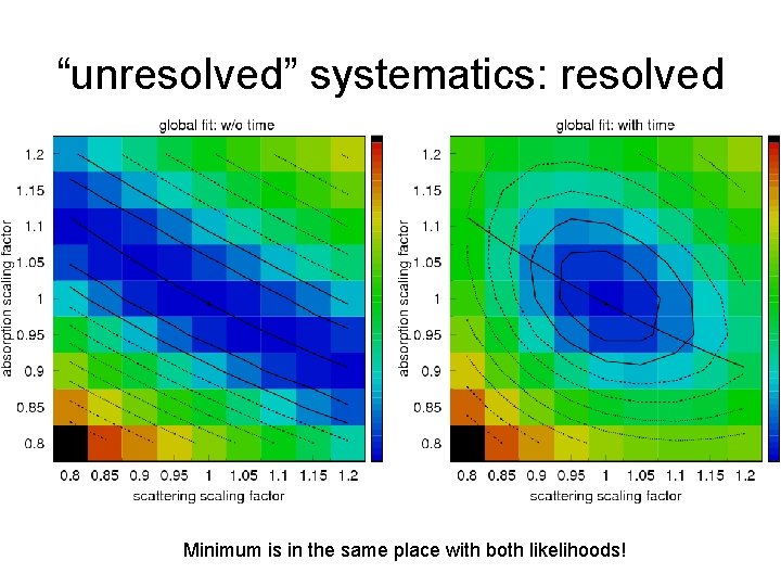
New global fit to everything in SPICE 1. For some starting values, find best values of lsca ~ labs. Charge only py photon yield factor toff global time offset (rising edge of the flasher pulse) f. SAM fraction of SAM contribution to the scattering function asca scaling of scattering coefficient aabs scaling of absorption coefficient 3. Repeat until converged (~3 iterations) 4. Refine the fit with lsca and labs independent from each other Full likelihood with timing 2. Find best values of py, toff, f. SAM, asca, aabs, llhtot, …

Verification with toy simulation Input table Simulated 60 x 250 events Reconstructed table with 10 event/flasher 250 event/flasher In the dust peak

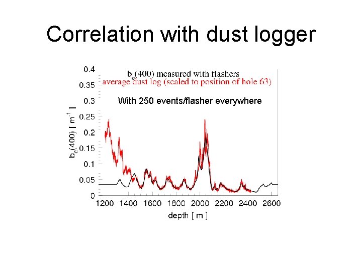
Correlation with dust logger With 10250 events/flasher, events/flasher 250 everywhere in dust peak

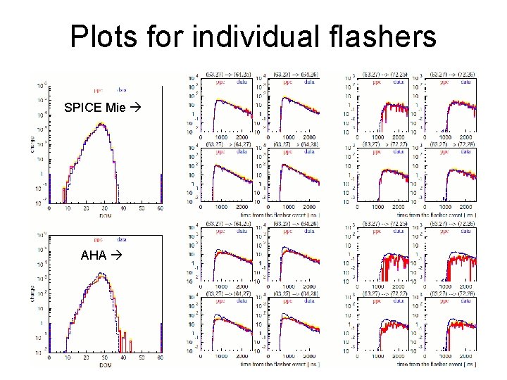
Plots for individual flashers SPICE Mie AHA

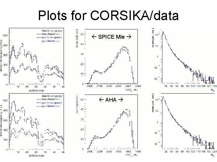
Plots for CORSIKA/data SPICE Mie AHA

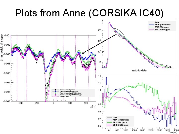
Plots from Anne (CORSIKA IC 40)

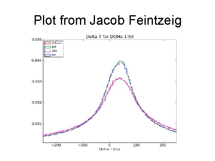
Plot from Jacob Feintzeig

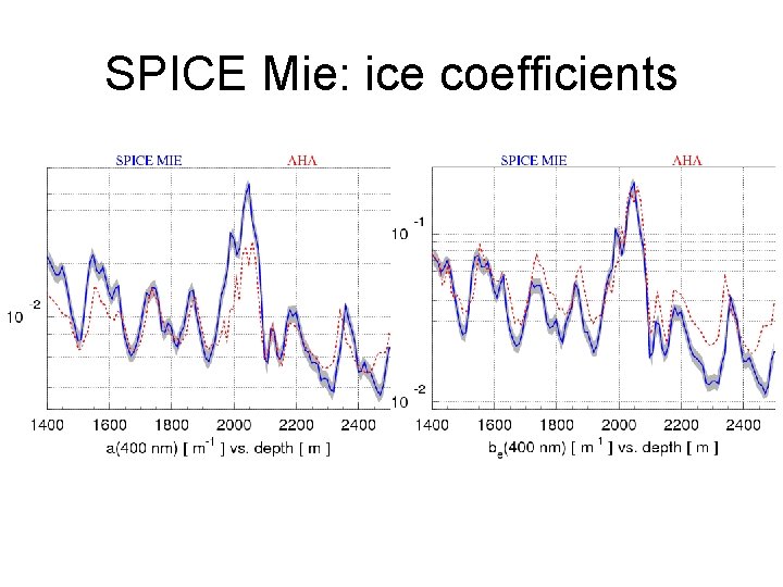
SPICE Mie: ice coefficients

“unresolved” systematics: resolved Minimum is in the same place with both likelihoods!

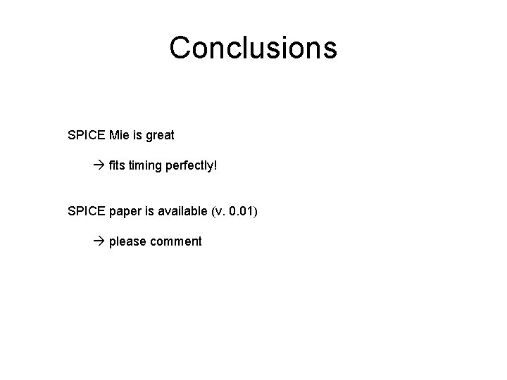
Conclusions SPICE Mie is great fits timing perfectly! SPICE paper is available (v. 0. 01) please comment