Spending and the Exchange Rate in the Keynesian

Spending and the Exchange Rate in the Keynesian Model Caves, Frankel and Jones (2007) World Trade and Payments, 10 e, Pearson Course in International finance International Master in Quantitative Finance

Outline • Transmission of disturbances under different FX regimes • Expenditure-switching and Expenditure-reducing policies – – • Types of policies SWAN diagram Monetary factors – IS-LM curve – Policy options: monetary expansion, fiscal expansion and/or devaluation

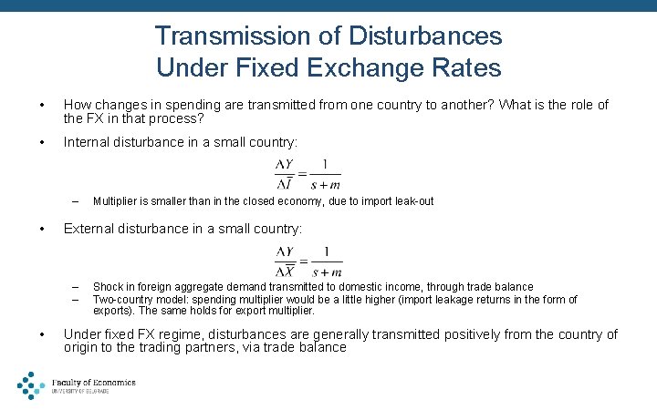
Transmission of Disturbances Under Fixed Exchange Rates • How changes in spending are transmitted from one country to another? What is the role of the FX in that process? • Internal disturbance in a small country: – • External disturbance in a small country: – – • Multiplier is smaller than in the closed economy, due to import leak-out Shock in foreign aggregate demand transmitted to domestic income, through trade balance Two-country model: spending multiplier would be a little higher (import leakage returns in the form of exports). The same holds for export multiplier. Under fixed FX regime, disturbances are generally transmitted positively from the country of origin to the trading partners, via trade balance

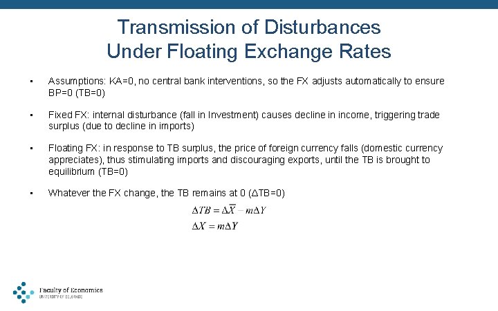
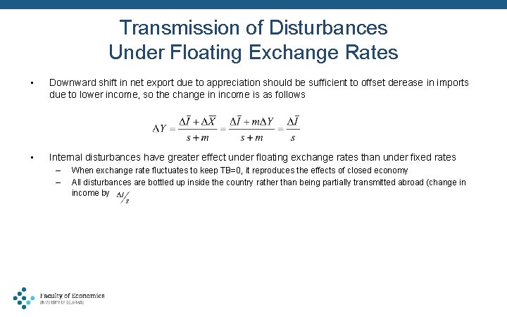
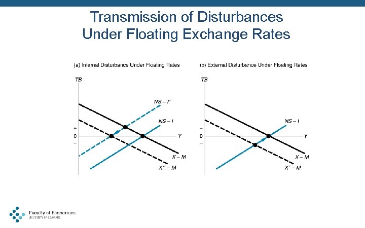
Transmission of Disturbances Under Floating Exchange Rates • Assumptions: KA=0, no central bank interventions, so the FX adjusts automatically to ensure BP=0 (TB=0) • Fixed FX: internal disturbance (fall in Investment) causes decline in income, triggering trade surplus (due to decline in imports) • Floating FX: in response to TB surplus, the price of foreign currency falls (domestic currency appreciates), thus stimulating imports and discouraging exports, until the TB is brought to equilibrium (TB=0) • Whatever the FX change, the TB remains at 0 (ΔTB=0)

Transmission of Disturbances Under Floating Exchange Rates • Downward shift in net export due to appreciation should be sufficient to offset derease in imports due to lower income, so the change in income is as follows • Internal disturbances have greater effect under floating exchange rates than under fixed rates – – When exchange rate fluctuates to keep TB=0, it reproduces the effects of closed economy All disturbances are bottled up inside the country rather than being partially transmitted abroad (change in income by

Transmission of Disturbances Under Floating Exchange Rates

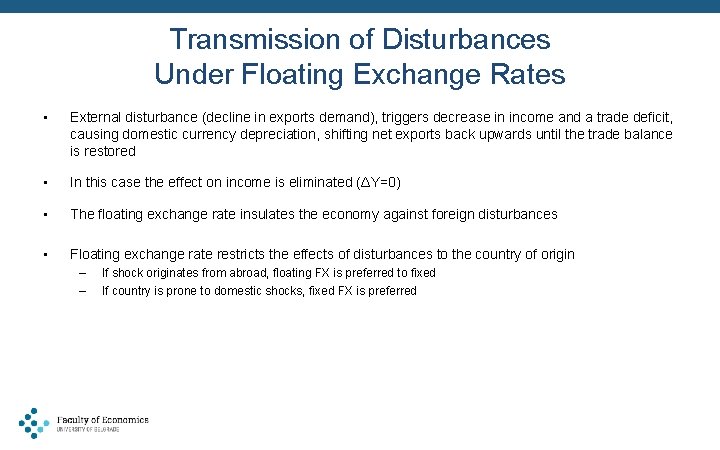
Transmission of Disturbances Under Floating Exchange Rates • External disturbance (decline in exports demand), triggers decrease in income and a trade deficit, causing domestic currency depreciation, shifting net exports back upwards until the trade balance is restored • In this case the effect on income is eliminated (ΔY=0) • The floating exchange rate insulates the economy against foreign disturbances • Floating exchange rate restricts the effects of disturbances to the country of origin – – If shock originates from abroad, floating FX is preferred to fixed If country is prone to domestic shocks, fixed FX is preferred

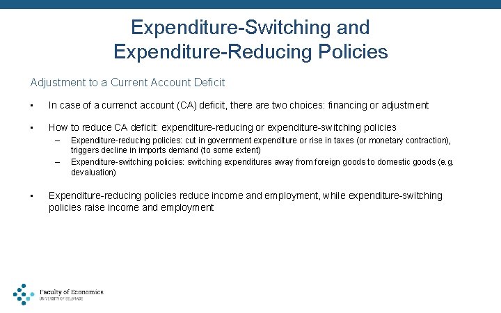
Expenditure-Switching and Expenditure-Reducing Policies Adjustment to a Current Account Deficit • In case of a currenct account (CA) deficit, there are two choices: financing or adjustment • How to reduce CA deficit: expenditure-reducing or expenditure-switching policies – – • Expenditure-reducing policies: cut in government expenditure or rise in taxes (or monetary contraction), triggers decline in imports demand (to some extent) Expenditure-switching policies: switching expenditures away from foreign goods to domestic goods (e. g. devaluation) Expenditure-reducing policies reduce income and employment, while expenditure-switching policies raise income and employment

Expenditure-Switching and Expenditure-Reducing Policies Types of Expenditure-Switching policies • Price deflation – Due to minimum wage laws, unions, contracts, etc. this option is usually rulled out • Devaluation • Direct trade controls (tarrifs or exports subsidies) – – • Nontarrif barriers (quantitative restrictions or quotas) – • 10% tarrifs + 10% exports subsidies = 10% devaluation (in terms of relative prices) e. g. Smoot-Hawley tarrif in the USA in 1930 s („beggar-thy-neighbour“ policies), which has triggered strategic response of trade partners, leading to collapse of world trade. After WWII GATT was set to reduce the tarrifs Tarrifs yield tax revenues, thus inducing expenditure-reducing effects, while quotas have only expenditureswitching effects, which is why tarrifs are more efficient Advanced deposits on imports – The same effect as tarrifs („tarrif“ equal to the interest on deposited money), thus triggering also expenditurereducing effects

Expenditure-Switching and Expenditure-Reducing Policies • The two-tier exchange rate – – • Capital controls – – • One exchange rate for current account transactions (fixed FX) and another one for capital-account transactions (market-based FX) Difficult to administer (spillover effects from current account to capital account FX market) …keep capital from moving where it earnes a higher return. If the difference in returns faced by lender is a difference in real social productivity, then there are social welfare costs When the central bank is influencing the price of credit, the connection between the market price and social productivity is no longer certain Multiple exchange rates – Using alternative exchange rate for imports of luxury goods

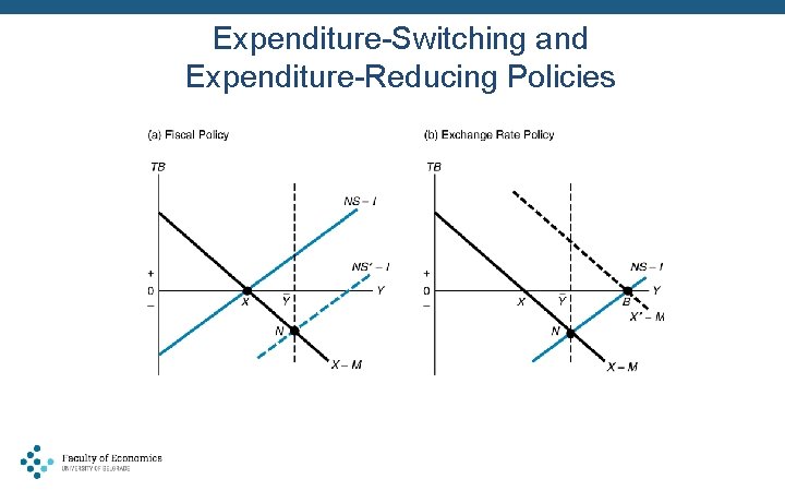
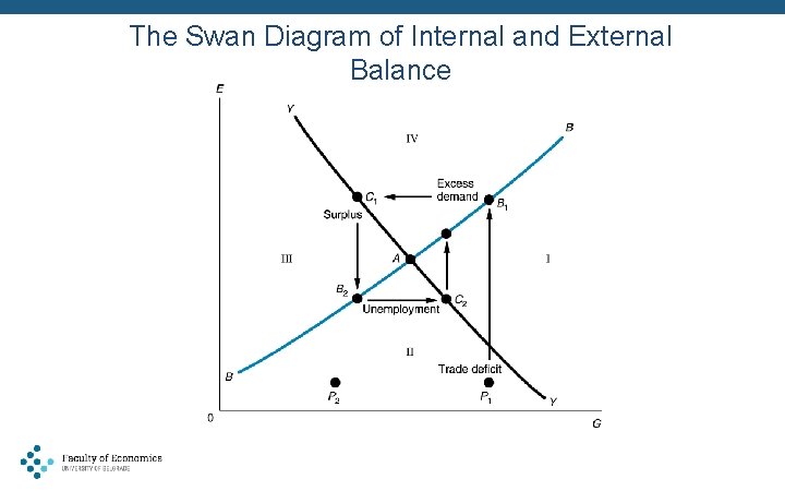
Expenditure-Switching and Expenditure-Reducing Policies THE SWAN DIAGRAM • Two policy goals – – • external balance (TB=0) Internal balance (output equal to full employemnt or to potential output) Expansionary fiscal policy leads to internal balance, but triggers external balance – The opposite holds for contractionary fiscal policy • • Devaluation raises output and improves trade balance – – • What determines the efficiency of fiscal policy in providing internal balance? Revaluation leads to internal balance at the expense of external imbalance Devaluation leads to external balance, but at the expense of internal imbalance Two policy goals require two policy tools (Tinbergen; Meade, Mundell) – – Expenditure switching (devaluation), and Expenditure reducing (government expenditure)

Expenditure-Switching and Expenditure-Reducing Policies

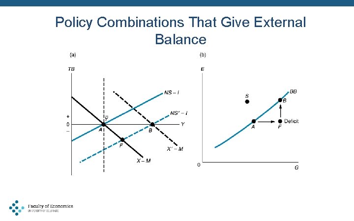
Expenditure-Switching and Expenditure-Reducing Policies THE SWAN DIAGRAM: EXTERNAL IMBALANCE • Another option – starting point is external and internal balance – If government increases expenditures, it must devalue to maintain external imbalance • • If the economy is not in balance (e. g. any point off the BB line), E is to low or G is to high for external balance (TB<0) – – • For TB=0, both G and E must vary together (BB upward sloping line) It is necessary to cut G or to increase E, in order to restore external balance The opposite holds if TB>0 (point S) Only under floating FX regime will the economy be at the BB line, as the FX adjusts automatically to maintain external balance

Policy Combinations That Give External Balance

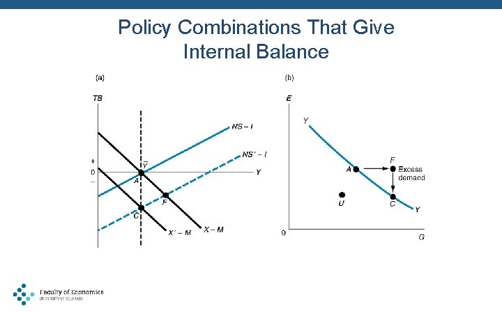
Expenditure-Switching and Expenditure-Reducing Policies THE SWAN DIAGRAM: INTERNAL IMBALANCE • Starting from external and internal balance and than changing G, means that E must also change in the reverse manner, to maintain balance – – – • Rise in G implies the need for revaluation Higher G must be accompanied by a lower E Internal balance maintained at YY curve If the economy is not in internal balance (e. g. any point off the YY line), E is to high or G is to low for internal balance – – It is necessary to cut G or to reduce E (to decreasse foreign demand), in order to restore internal balance The opposite holds if there is a missing demand

Policy Combinations That Give Internal Balance

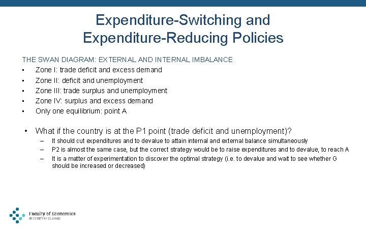
Expenditure-Switching and Expenditure-Reducing Policies THE SWAN DIAGRAM: EXTERNAL AND INTERNAL IMBALANCE • Zone I: trade deficit and excess demand • Zone II: deficit and unemployment • Zone III: trade surplus and unemployment • Zone IV: surplus and excess demand • Only one equilibrium: point A • What if the country is at the P 1 point (trade deficit and unemployment)? – – – It should cut expenditures and to devalue to attain internal and external balance simultaneously P 2 is almost the same case, but the correct strategy would be to raise expenditures and to devalue, to reach A It is a matter of experimentation to discover the optimal strategy (i. e. to devalue and wait to see whether G should be increased or decreased)

The Swan Diagram of Internal and External Balance

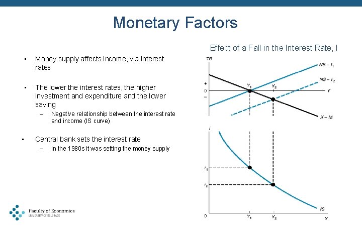
Monetary Factors Effect of a Fall in the Interest Rate, I • Money supply affects income, via interest rates • The lower the interest rates, the higher investment and expenditure and the lower saving – • Negative relationship between the interest rate and income (IS curve) Central bank sets the interest rate – In the 1980 s it was setting the money supply

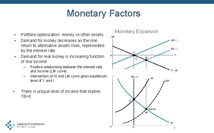
Monetary Factors • • • Portfolio optimization: money vs other assets Demand for money decreases as the real return to alternative assets rises, represented by the interest rate Demand for real money is increasing function of real income – – • Positive relationship between the interest rate and income (LM curve) Intersection of IS and LM curve gives equilibrium level of Y and I There is unique level of income that implies TB=0 Monetary Expansion

Monetary Factors • IS-LM equilibrium at the point which implies TB=0 • Three policy options: monetary expansion, fiscal expansion and devaluation MONETARY EXPANSION • Monetary expansion shifts LM curve to the right (fall in interest rate and rise in Y), i. e. fall in interest rate encourages investments and thus triggering rise in income – – New equilibrium is at point M The higher level of expenditure induced by monetary expansion has shifted a country to the trade deficit

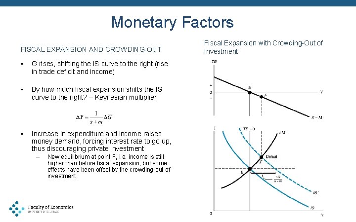
Monetary Factors FISCAL EXPANSION AND CROWDING-OUT • G rises, shifting the IS curve to the right (rise in trade deficit and income) • By how much fiscal expansion shifts the IS curve to the right? – Keynesian multiplier • Increase in expenditure and income raises money demand, forcing interest rate to go up, thus discouraging private investment – New equilibrium at point F, i. e. income is still higher than before fiscal expansion, but some effects have been offset by the crowding-out of investment Fiscal Expansion with Crowding-Out of Investment

Monetary Factors LIQUIDITY TRAP AND JAPAN IN THE 1990 s • Keynesian model neglects the effects of fiscal expansion on inflation, interest rates and rising public debt • …but it showed to be relevant in the Japan crisis in 1990 s – – • Colapse of stock and real estate bubble triggering deflation, unemployment and slow growth, but the goods prices did not decline enough to restore equilibrium Bank of Japan reduced interest rate to zero: further increases in money supply absorbed by the public withouth bringing reduction of the interest rate – liquidity trap • LM curve became flat Two important implications: – – Monetary policy becomes ineffective Fiscal policy becomes more effective • • As LM curve is flat, fiscal expansion triggers no increase in the interest rate to crowd out private investment – full mupltiplier shows up In 1997 the government raised taxes to cut the deficit, which pushed the economy back to recession

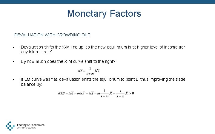
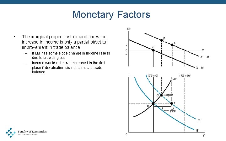
Monetary Factors DEVALUATION WITH CROWDING OUT • Devaluation shifts the X-M line up, so the new equilibrium is at higher level of income (for any interest rate) • By how much does the X-M curve shift to the right? • If LM curve was flat, devaluation shifts the equilibrium to point L, thus improving the trade balance by:

Monetary Factors • The marginal propensity to import times the increase in income is only a partial offset to improvement in trade balance – – If LM has some slope change in income is less due to crowding out Income would not have increased in the first place if devaluation did not stimulate trade balance