Soc 3306 a Lecture 10 Multivariate 3 Types

Soc 3306 a Lecture 10: Multivariate 3 Types of Relationships in Multiple Regression

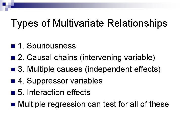
Types of Multivariate Relationships 1. Spuriousness n 2. Causal chains (intervening variable) n 3. Multiple causes (independent effects) n 4. Suppressor variables n 5. Interaction effects n Multiple regression can test for all of these n

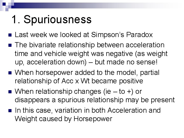
1. Spuriousness n n n Last week we looked at Simpson’s Paradox The bivariate relationship between acceleration time and vehicle weight was negative (as weight up, acceleration down) – but made no sense! When horsepower added to the model, partial relationship of Acc x Wt became positive When relationship changes (ie – to +) or disappears a spurious relationship may be present In this case, variation in both Acceleration and Weight caused by Horsepower

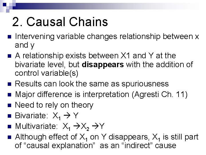
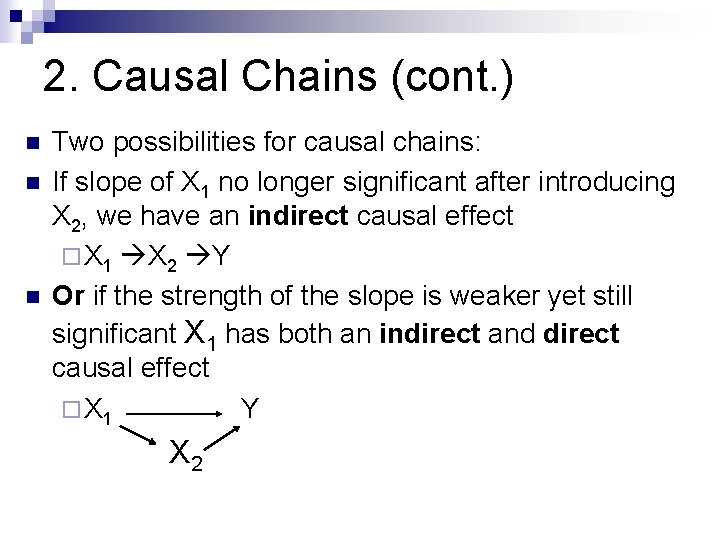
2. Causal Chains n n n n Intervening variable changes relationship between x and y A relationship exists between X 1 and Y at the bivariate level, but disappears with the addition of control variable(s) Results can look the same as spuriousness Major difference is interpretation (Agresti Ch. 11) Need to rely on theory Bivariate: X 1 Y Multivariate: X 1 X 2 Y Although effect of X 1 on Y disappears, X 1 is still part of “causal explanation” as an “indirect” cause

2. Causal Chains (cont. ) n n n Two possibilities for causal chains: If slope of X 1 no longer significant after introducing X 2, we have an indirect causal effect ¨ X 1 X 2 Y Or if the strength of the slope is weaker yet still significant X 1 has both an indirect and direct causal effect ¨ X 1 Y X 2

3. Multiple Causes Y (DV) has multiple causes n Independent variables have relatively separate effects on the dependent variable n Introduction of controls does little to change bivariate correlations and the bivariate slopes stay similar n Compare bivariate to partial correlations in multiple model and compare slopes in the bivariate and multiple models n

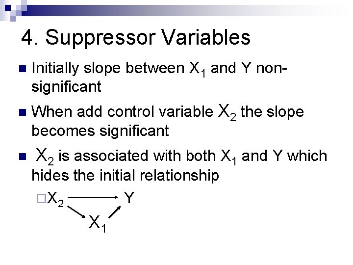
4. Suppressor Variables n Initially slope between X 1 and Y nonsignificant n When add control variable X 2 the slope becomes significant n X 2 is associated with both X 1 and Y which hides the initial relationship ¨X 2 Y X 1

4. Interactions n n n Not all IV effects on Y are independent and often IV’s interact with one another in their effect on Y Usually suggested by theory An interaction is present when you enter control variable and the original bivariate association differs by level of the control variable Does the slope of X 1 differ by category of X 2 when explaining Y? Can test this by introducing “interaction terms” into the multiple regression model (see Agresti Ch. 11 p. 340 – 343)

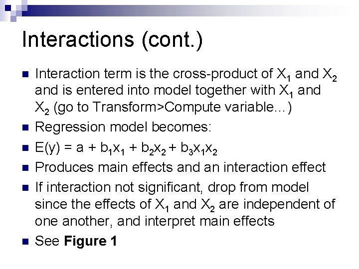
Interactions (cont. ) n n n Interaction term is the cross-product of X 1 and X 2 and is entered into model together with X 1 and X 2 (go to Transform>Compute variable…) Regression model becomes: E(y) = a + b 1 x 1 + b 2 x 2 + b 3 x 1 x 2 Produces main effects and an interaction effect If interaction not significant, drop from model since the effects of X 1 and X 2 are independent of one another, and interpret main effects See Figure 1

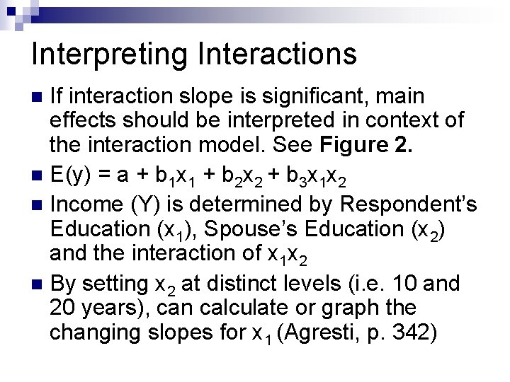
Interpreting Interactions If interaction slope is significant, main effects should be interpreted in context of the interaction model. See Figure 2. n E(y) = a + b 1 x 1 + b 2 x 2 + b 3 x 1 x 2 n Income (Y) is determined by Respondent’s Education (x 1), Spouse’s Education (x 2) and the interaction of x 1 x 2 n By setting x 2 at distinct levels (i. e. 10 and 20 years), can calculate or graph the changing slopes for x 1 (Agresti, p. 342) n