Soc 3306 a Lecture 9 Multivariate 2 More

Soc 3306 a Lecture 9: Multivariate 2 More on Multiple Regression: Building a Model and Interpreting Coefficients

Assumptions for Multiple Regression Random sample n Distribution of y is relatively normal n ¨ Check n histogram Standard deviation of y is constant for each value of x ¨ Check scatterplots (Figure 1)

Problems to Watch For… Violation of assumptions, especially normality of DV and heteroscedasticity (Figure 1) n Simpson’s Paradox n Multicollinearity n

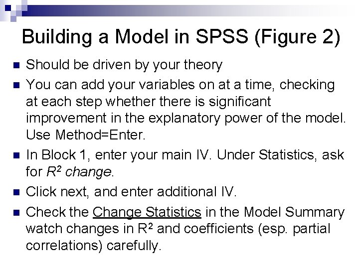
Building a Model in SPSS (Figure 2) n n n Should be driven by your theory You can add your variables on at a time, checking at each step whethere is significant improvement in the explanatory power of the model. Use Method=Enter. In Block 1, enter your main IV. Under Statistics, ask for R 2 change. Click next, and enter additional IV. Check the Change Statistics in the Model Summary watch changes in R 2 and coefficients (esp. partial correlations) carefully.

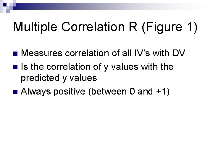
Multiple Correlation R (Figure 1) Measures correlation of all IV’s with DV n Is the correlation of y values with the predicted y values n Always positive (between 0 and +1) n

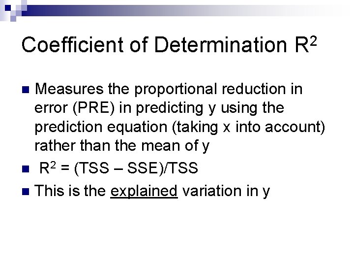
Coefficient of Determination R 2 Measures the proportional reduction in error (PRE) in predicting y using the prediction equation (taking x into account) rather than the mean of y n R 2 = (TSS – SSE)/TSS n This is the explained variation in y n

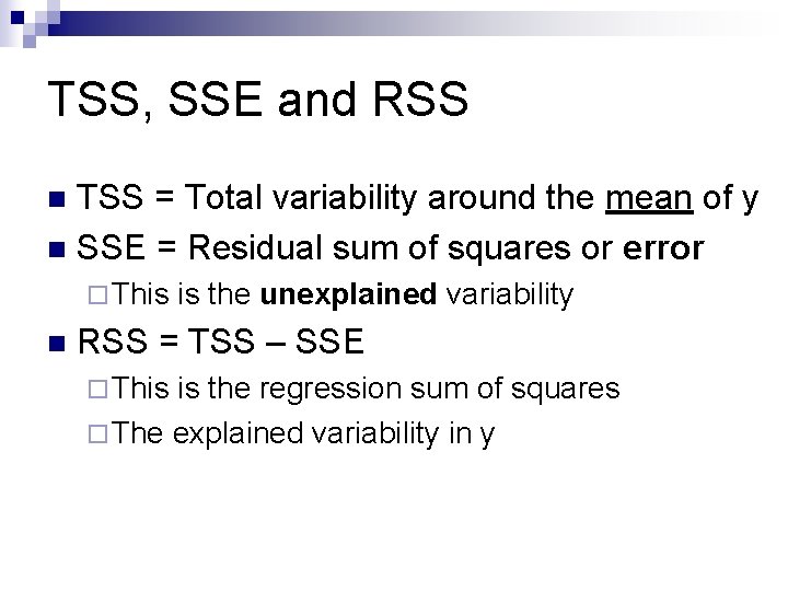
TSS, SSE and RSS TSS = Total variability around the mean of y n SSE = Residual sum of squares or error n ¨ This n is the unexplained variability RSS = TSS – SSE ¨ This is the regression sum of squares ¨ The explained variability in y

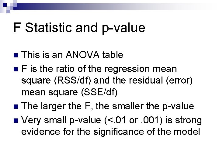
F Statistic and p-value This is an ANOVA table n F is the ratio of the regression mean square (RSS/df) and the residual (error) mean square (SSE/df) n The larger the F, the smaller the p-value n Very small p-value (<. 01 or. 001) is strong evidence for the significance of the model n

Slope (b), β, t-statistic and p-value n n n Slope is measured in actual units of variables. Change in y for 1 unit of x In multiple regression, each slope is controlled for all other x variables β is standardized slope – can compare strength t = b/se with df= n-(k+1), note: k = # of predictors Small p-value indicates significant relationship with y, controlling for other variables in model Note: in bivariate regression, t 2 = F and β = r

Simpson’s Paradox (Figure 3) Indicates a spurious relationship n See printouts in Figure 1 n Indicated by change in the sign of partial correlations n Can also check the partial regression plots (ask for all partial plots under Plots) n

Multicollinearity (Figure 1 and 2) n n n Two independent variables in the model, i. e. x 1 and x 2, are correlated with y but also highly correlated (>. 700) with each other Both are explaining the same proportion of variation in y but adding x 2 to the model does not increase explanatory value (R, R 2) Check correlation between IV’s in correlation matrix. Ask for and check partial correlations in multiple regression (Part and Partial under Statistics) If partial correlation in multiple model much lower than bivariate correlation, multicollinearity indicated

A Few Tips for SPSS Mini 6 n n n Review powerpoint for Lectures 8 and 9 Read assignment over carefully before starting. When creating your model, build your model carefully one block at a time. Watch for spurious relationships. Revise model if needed. Drop any unnecessary variables (i. e. evidence of multicollinearity or new variables that do not appreciably increase R 2. ) Keep your model simple. Aim for good explanatory value with the least variables possible.