q OR1 Opt 2018 1 q OR1 Opt

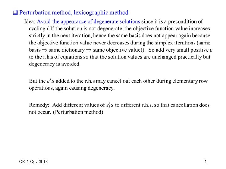
q OR-1 Opt. 2018 1

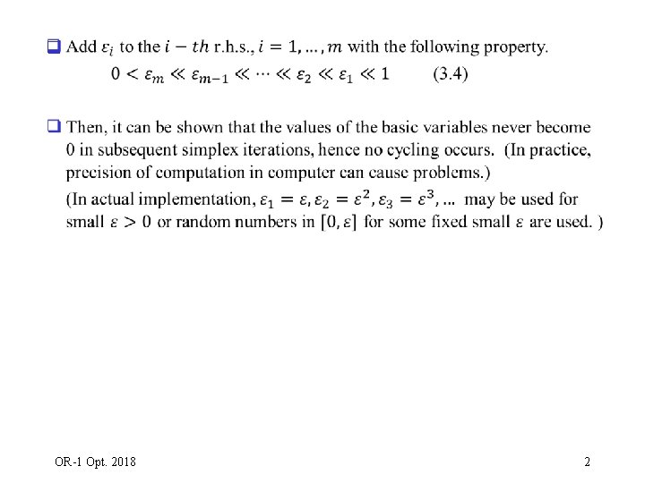
q OR-1 Opt. 2018 2

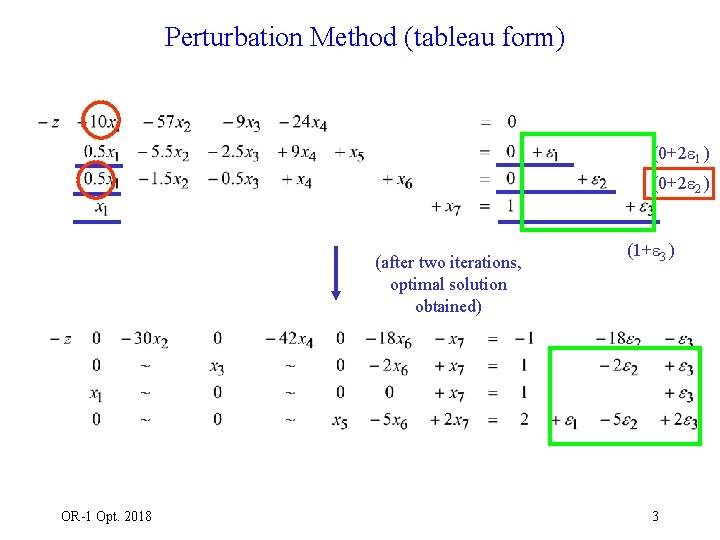
Perturbation Method (tableau form) (0+2 1 ) (0+2 2 ) (after two iterations, optimal solution obtained) OR-1 Opt. 2018 (1+ 3 ) 3

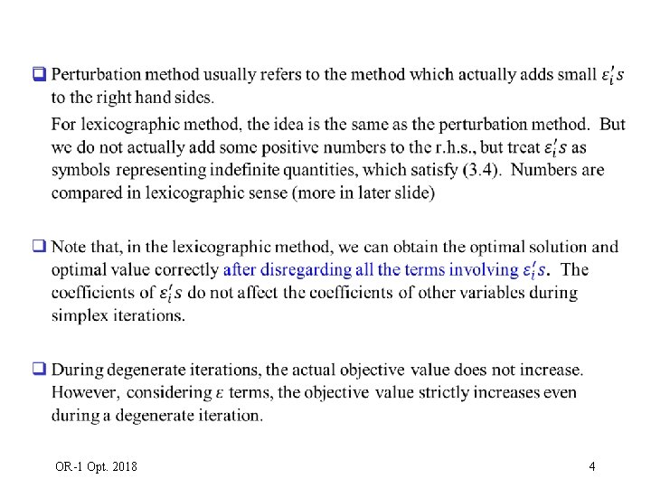
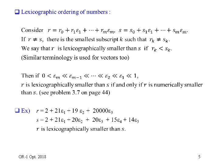
q OR-1 Opt. 2018 4

q OR-1 Opt. 2018 5

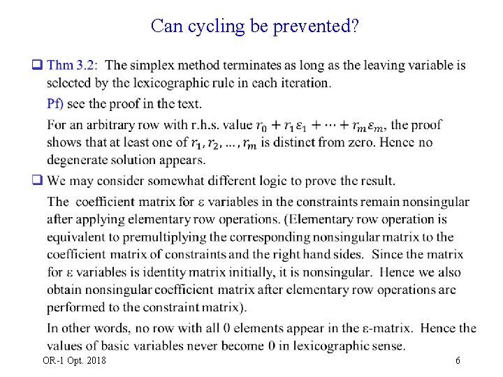
Can cycling be prevented? q OR-1 Opt. 2018 6

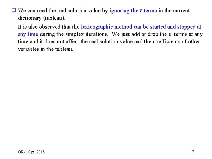
q We can read the real solution value by ignoring the terms in the current dictionary (tableau). It is also observed that the lexicographic method can be started and stopped at any time during the simplex iterations. We just add or drop the terms at any time and it does not affect the real solution value and the coefficients of other variables in the tableau. OR-1 Opt. 2018 7

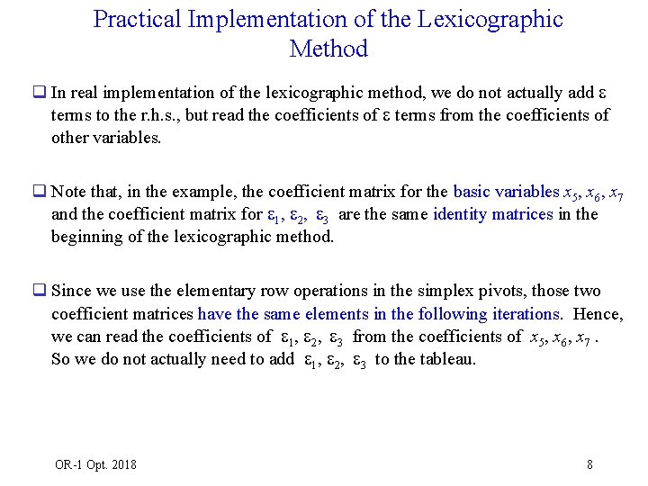
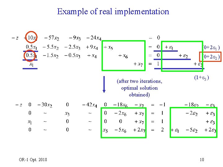
Practical Implementation of the Lexicographic Method q In real implementation of the lexicographic method, we do not actually add terms to the r. h. s. , but read the coefficients of terms from the coefficients of other variables. q Note that, in the example, the coefficient matrix for the basic variables x 5, x 6, x 7 and the coefficient matrix for 1, 2, 3 are the same identity matrices in the beginning of the lexicographic method. q Since we use the elementary row operations in the simplex pivots, those two coefficient matrices have the same elements in the following iterations. Hence, we can read the coefficients of 1, 2, 3 from the coefficients of x 5, x 6, x 7. So we do not actually need to add 1, 2, 3 to the tableau. OR-1 Opt. 2018 8

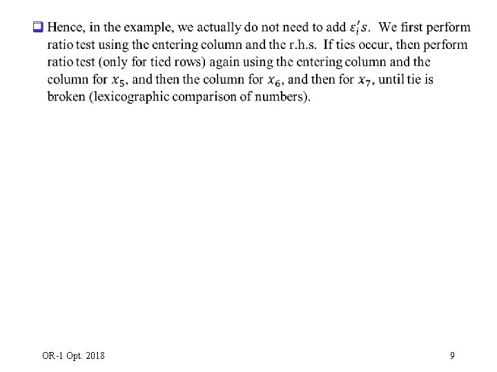
q OR-1 Opt. 2018 9

Example of real implementation (0+2 1 ) (0+2 2 ) (after two iterations, optimal solution obtained) OR-1 Opt. 2018 (1+ 3 ) 10

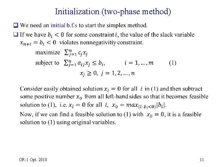
Initialization (two-phase method) q OR-1 Opt. 2018 11

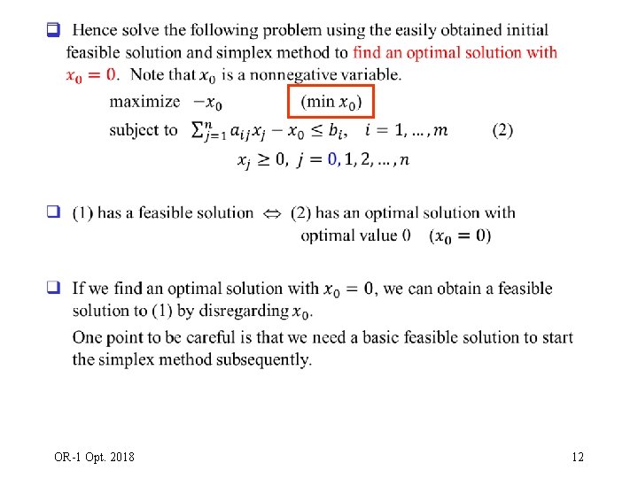
q OR-1 Opt. 2018 12

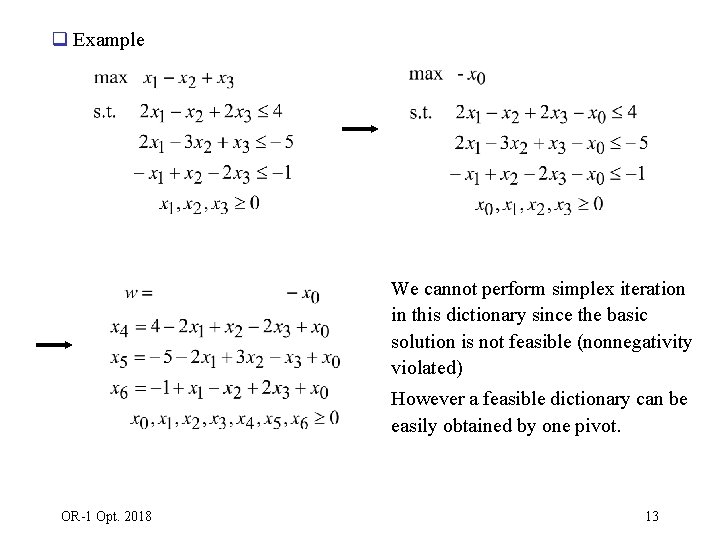
q Example We cannot perform simplex iteration in this dictionary since the basic solution is not feasible (nonnegativity violated) However a feasible dictionary can be easily obtained by one pivot. OR-1 Opt. 2018 13

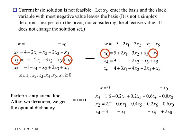
q Perform simplex method. After two iterations, we get the optimal dictionary OR-1 Opt. 2018 14

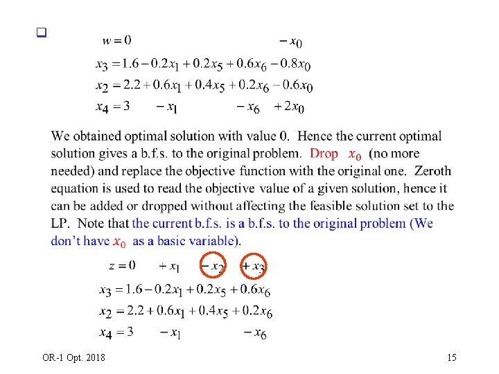
q OR-1 Opt. 2018 15

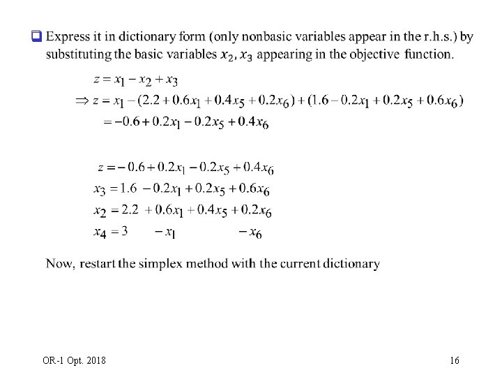
q OR-1 Opt. 2018 16

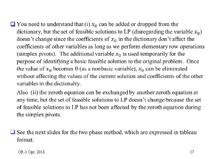
q OR-1 Opt. 2018 17

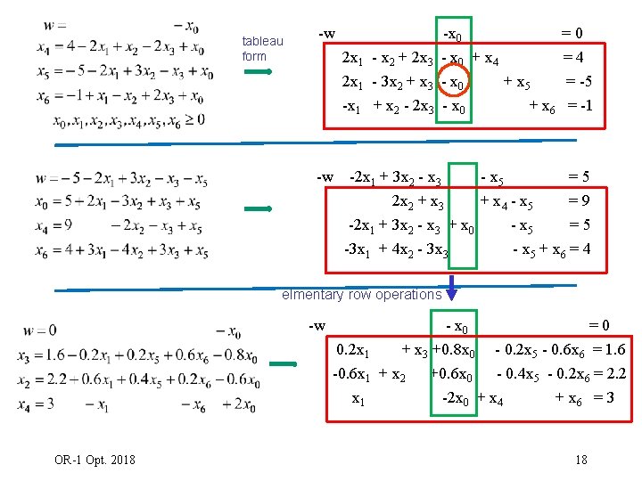
tableau form -w -x 0 2 x 1 - x 2 + 2 x 3 - x 0 + x 4 2 x 1 - 3 x 2 + x 3 - x 0 + x 5 -x 1 + x 2 - 2 x 3 - x 0 + x 6 =0 =4 = -5 = -1 -w -2 x 1 + 3 x 2 - x 3 - x 5 =5 2 x 2 + x 3 + x 4 - x 5 =9 -2 x 1 + 3 x 2 - x 3 + x 0 - x 5 =5 -3 x 1 + 4 x 2 - 3 x 3 - x 5 + x 6 = 4 elmentary row operations -w OR-1 Opt. 2018 - x 0 =0 0. 2 x 1 + x 3 +0. 8 x 0 - 0. 2 x 5 - 0. 6 x 6 = 1. 6 -0. 6 x 1 + x 2 +0. 6 x 0 - 0. 4 x 5 - 0. 2 x 6 = 2. 2 x 1 -2 x 0 + x 4 + x 6 = 3 18

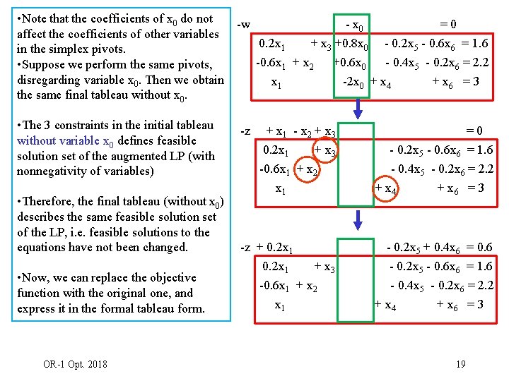
• Note that the coefficients of x 0 do not -w - x 0 =0 affect the coefficients of other variables 0. 2 x 1 + x 3 +0. 8 x 0 - 0. 2 x 5 - 0. 6 x 6 = 1. 6 in the simplex pivots. -0. 6 x 1 + x 2 +0. 6 x 0 - 0. 4 x 5 - 0. 2 x 6 = 2. 2 • Suppose we perform the same pivots, disregarding variable x 0. Then we obtain x 1 -2 x 0 + x 4 + x 6 = 3 the same final tableau without x 0. • The 3 constraints in the initial tableau without variable x 0 defines feasible solution set of the augmented LP (with nonnegativity of variables) • Therefore, the final tableau (without x 0) describes the same feasible solution set of the LP, i. e. feasible solutions to the equations have not been changed. • Now, we can replace the objective function with the original one, and express it in the formal tableau form. OR-1 Opt. 2018 -z + x 1 - x 2 + x 3 0. 2 x 1 + x 3 -0. 6 x 1 + x 2 x 1 =0 - 0. 2 x 5 - 0. 6 x 6 = 1. 6 - 0. 4 x 5 - 0. 2 x 6 = 2. 2 + x 4 + x 6 = 3 -z + 0. 2 x 1 + x 3 -0. 6 x 1 + x 2 x 1 - 0. 2 x 5 + 0. 4 x 6 = 0. 6 - 0. 2 x 5 - 0. 6 x 6 = 1. 6 - 0. 4 x 5 - 0. 2 x 6 = 2. 2 + x 4 + x 6 = 3 19

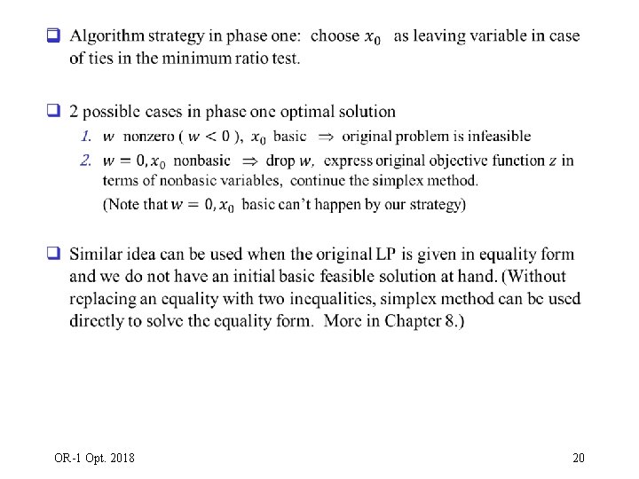
q OR-1 Opt. 2018 20

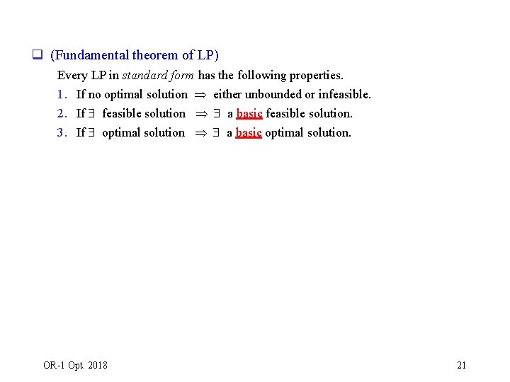
q (Fundamental theorem of LP) Every LP in standard form has the following properties. 1. If no optimal solution either unbounded or infeasible. 2. If feasible solution a basic feasible solution. 3. If optimal solution a basic optimal solution. OR-1 Opt. 2018 21