Prejudice and Discrimination in Housing Allen C Goodman

Prejudice and Discrimination in Housing © Allen C. Goodman 2000

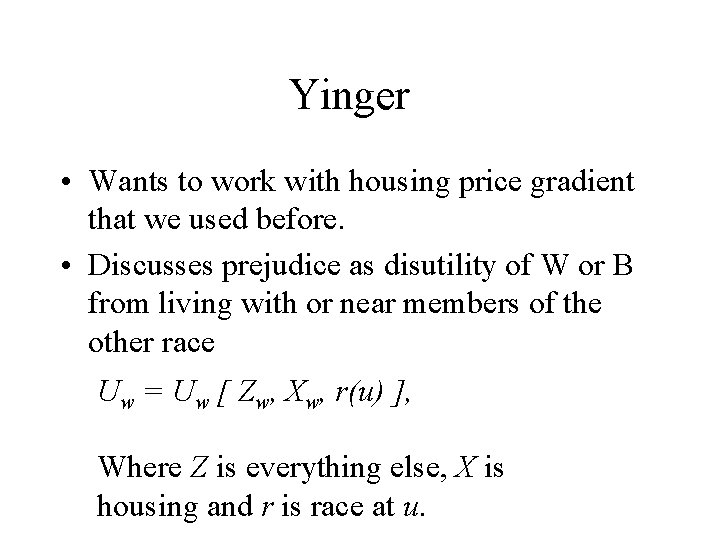
Yinger • Wants to work with housing price gradient that we used before. • Discusses prejudice as disutility of W or B from living with or near members of the other race Uw = Uw [ Zw, Xw, r(u) ], Where Z is everything else, X is housing and r is race at u.

Prejudice ONE FORM OF r(u) IS: Hw = Xw Dw [r(u)], WHERE Dw(0) = 1, D' < 0. 1 DW DB D*w REDEFINES TERMS AS: Hw = Hw [Xw, r(u)]. R = fraction B

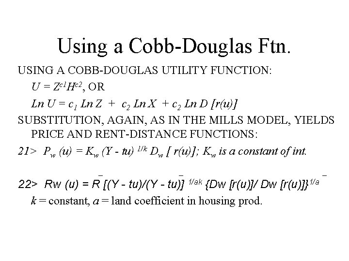
Using a Cobb-Douglas Ftn. USING A COBB-DOUGLAS UTILITY FUNCTION: U = Zc 1 Hc 2, OR Ln U = c 1 Ln Z + c 2 Ln X + c 2 Ln D [r(u)] SUBSTITUTION, AGAIN, AS IN THE MILLS MODEL, YIELDS PRICE AND RENT-DISTANCE FUNCTIONS: 21> Pw (u) = Kw (Y - tu) 1/k Dw [ r(u)]; Kw is a constant of int. _ _ 22> Rw (u) = R [(Y - tu)/(Y - tu)] 1/ak {Dw [r(u)]/ Dw [r(u)]}1/a k = constant, a = land coefficient in housing prod. _

For W, for B _ _ _ [r(u)]}1/a 22> Rw (u) = R [(Y - tu)/(Y - tu)] 1/ak {Dw [r(u)]/ Dw For prejudiced W, function must be lower at locations with higher concentration of B. Can come up with similar for B. Hb = Xb Db [r(u)], WHERE Db(1) = 1, D' > 0. _ _ 24> Rb (u) = R [(Y - tu)/(Y - tu)] 1/ak {Db [r(u)]/ Db _ [r(u)]}1/a

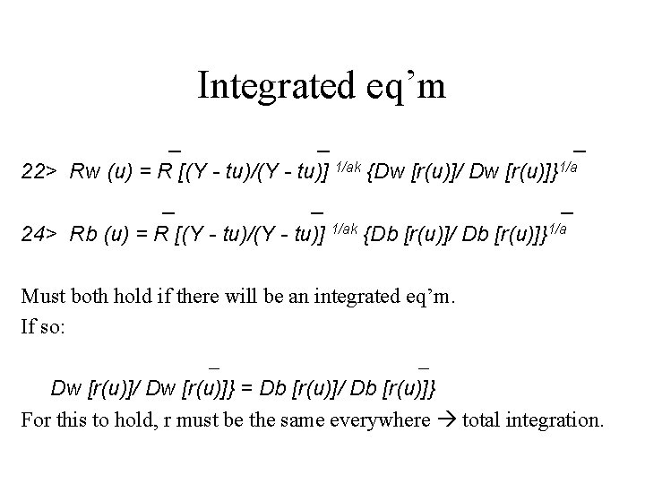
Integrated eq’m _ _ _ 22> Rw (u) = R [(Y - tu)/(Y - tu)] 1/ak {Dw [r(u)]/ Dw [r(u)]}1/a _ _ _ 24> Rb (u) = R [(Y - tu)/(Y - tu)] 1/ak {Db [r(u)]/ Db [r(u)]}1/a Must both hold if there will be an integrated eq’m. If so: _ _ Dw [r(u)]/ Dw [r(u)]} = Db [r(u)]/ Db [r(u)]} For this to hold, r must be the same everywhere total integration.

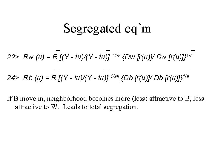
Segregated eq’m _ _ _ 22> Rw (u) = R [(Y - tu)/(Y - tu)] 1/ak {Dw [r(u)]/ Dw [r(u)]}1/a _ _ _ 24> Rb (u) = R [(Y - tu)/(Y - tu)] 1/ak {Db [r(u)]/ Db [r(u)]}1/a If B move in, neighborhood becomes more (less) attractive to B, less attractive to W. Leads to total segregation.

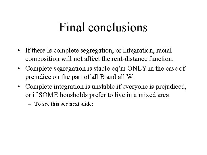
Final conclusions • If there is complete segregation, or integration, racial composition will not affect the rent-distance function. • Complete segregation is stable eq’m ONLY in the case of prejudice on the part of all B and all W. • Complete integration is unstable if everyone is prejudiced, or if SOME housholds prefer to live in a mixed area. – To see this see next slide:

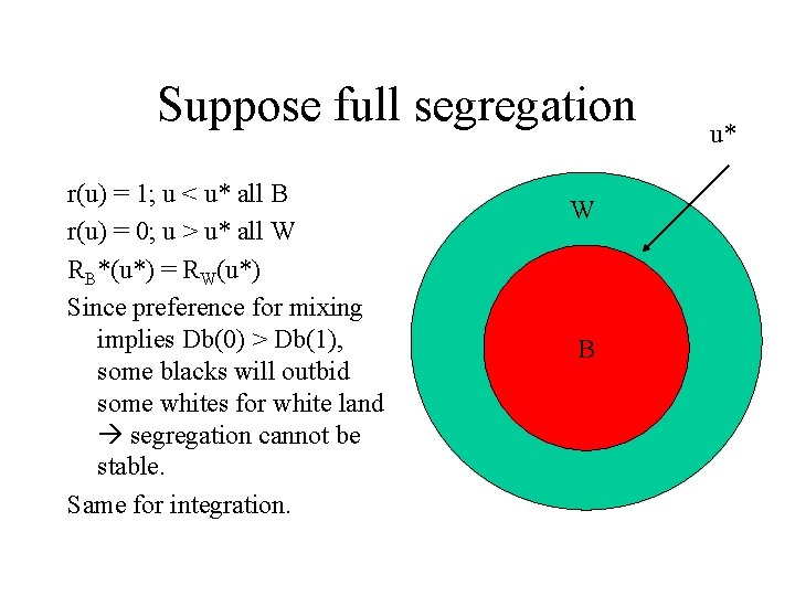
Suppose full segregation r(u) = 1; u < u* all B r(u) = 0; u > u* all W RB*(u*) = RW(u*) Since preference for mixing implies Db(0) > Db(1), some blacks will outbid some whites for white land segregation cannot be stable. Same for integration. W W B u*

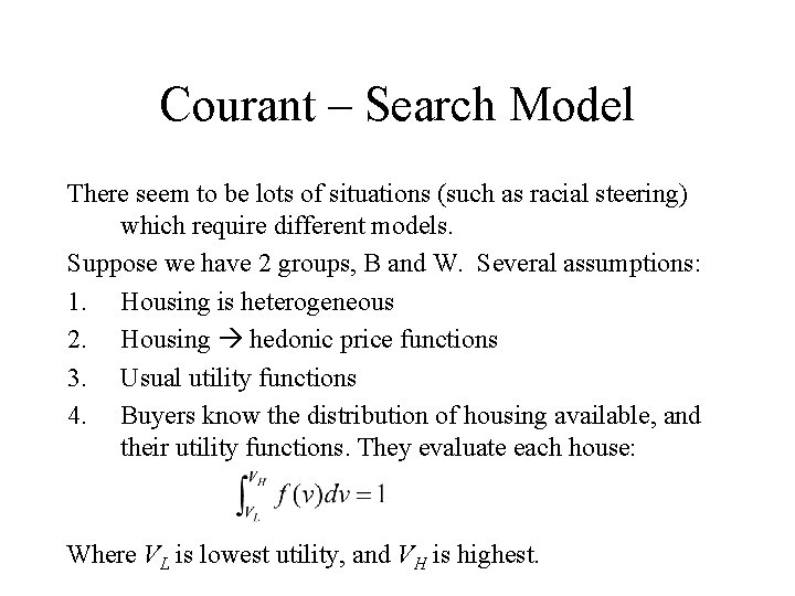
Courant – Search Model There seem to be lots of situations (such as racial steering) which require different models. Suppose we have 2 groups, B and W. Several assumptions: 1. Housing is heterogeneous 2. Housing hedonic price functions 3. Usual utility functions 4. Buyers know the distribution of housing available, and their utility functions. They evaluate each house: Where VL is lowest utility, and VH is highest.

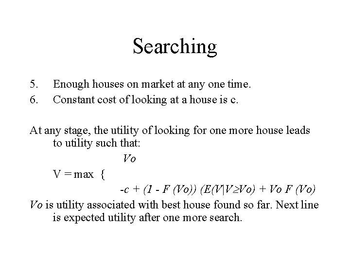
Searching 5. 6. Enough houses on market at any one time. Constant cost of looking at a house is c. At any stage, the utility of looking for one more house leads to utility such that: Vo V = max { -c + (1 - F (Vo)) (E(V|V Vo) + Vo F (Vo) Vo is utility associated with best house found so far. Next line is expected utility after one more search.

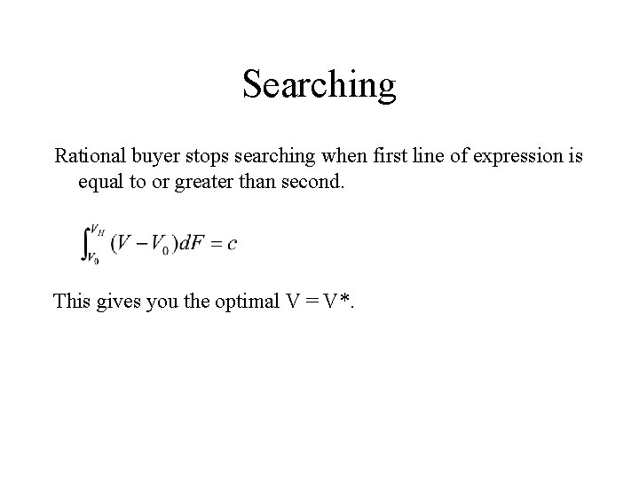
Searching Rational buyer stops searching when first line of expression is equal to or greater than second. This gives you the optimal V = V*.

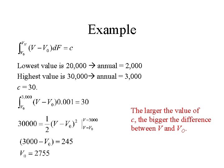
Example Lowest value is 20, 000 annual = 2, 000 Highest value is 30, 000 annual = 3, 000 c = 30. The larger the value of c, the bigger the difference between V and VO.

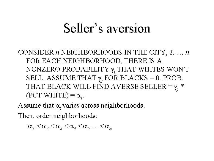
Seller’s aversion CONSIDER n NEIGHBORHOODS IN THE CITY, 1, . . . , n. FOR EACH NEIGHBORHOOD, THERE IS A NONZERO PROBABILITY j THAT WHITES WON'T SELL. ASSUME THAT j FOR BLACKS = 0. PROB. THAT BLACK WILL FIND AVERSE SELLER = j * (PCT WHITE) = j. Assume that j varies across neighborhoods. Then, order neighborhoods: 1 2 3 4 5 … n

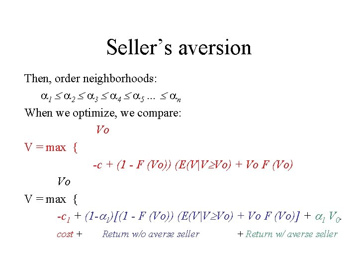
Seller’s aversion Then, order neighborhoods: 1 2 3 4 5 … n When we optimize, we compare: Vo V = max { -c + (1 - F (Vo)) (E(V|V Vo) + Vo F (Vo) Vo V = max { -c 1 + (1 - 1)[(1 - F (Vo)) (E(V|V Vo) + Vo F (Vo)] + 1 V 0. cost + Return w/o averse seller + Return w/ averse seller

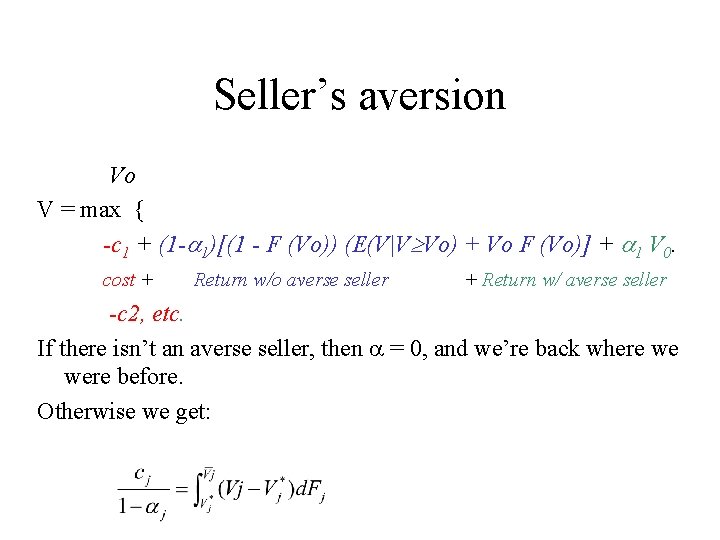
Seller’s aversion Vo V = max { -c 1 + (1 - 1)[(1 - F (Vo)) (E(V|V Vo) + Vo F (Vo)] + 1 V 0. cost + Return w/o averse seller + Return w/ averse seller -c 2, etc. If there isn’t an averse seller, then = 0, and we’re back where we were before. Otherwise we get:

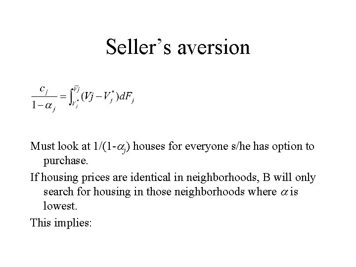
Seller’s aversion Must look at 1/(1 - j) houses for everyone s/he has option to purchase. If housing prices are identical in neighborhoods, B will only search for housing in those neighborhoods where is lowest. This implies:

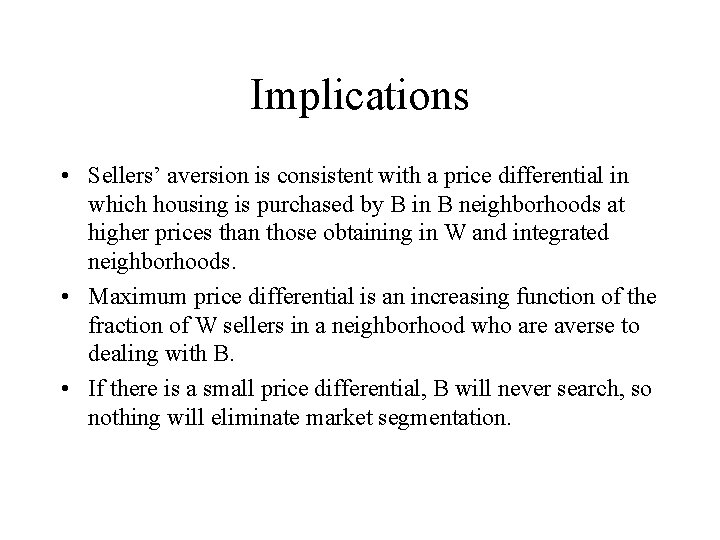
Implications • Sellers’ aversion is consistent with a price differential in which housing is purchased by B in B neighborhoods at higher prices than those obtaining in W and integrated neighborhoods. • Maximum price differential is an increasing function of the fraction of W sellers in a neighborhood who are averse to dealing with B. • If there is a small price differential, B will never search, so nothing will eliminate market segmentation.