Lee Carver Update 171111 JUAS Application Got accepted

Lee Carver - Update 17/11/11

JUAS Application • Got accepted onto JUAS with a scholarship to cover accommodation (400 Euros) • Monday 9 th January – Thursday 9 th February. • Programme found: https: //espace. cern. ch/juas/programmes 2011. aspx

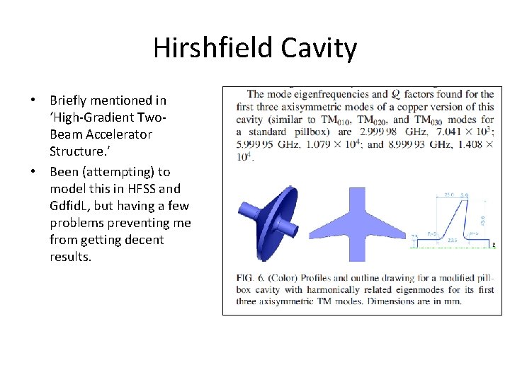
Hirshfield Cavity • Briefly mentioned in ‘High-Gradient Two. Beam Accelerator Structure. ’ • Been (attempting) to model this in HFSS and Gdfid. L, but having a few problems preventing me from getting decent results.

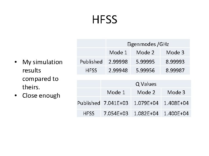
HFSS Eigenmodes /GHz Mode 1 Mode 2 Mode 3 • My simulation results compared to theirs. • Close enough Published 2. 99998 5. 99995 8. 99993 HFSS 2. 99948 5. 99956 8. 99987 Q Values Mode 2 Mode 3 Mode 1 Published 7. 041 E+03 1. 079 E+04 1. 408 E+04 HFSS 7. 054 E+03 1. 082 E+04 1. 400 E+04

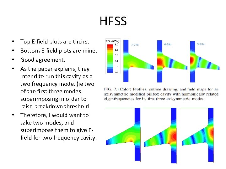
HFSS Top E-field plots are theirs. Bottom E-field plots are mine. Good agreement. As the paper explains, they intend to run this cavity as a two frequency mode. (ie two of the first three modes superimposing in order to raise breakdown threshold. • Therefore, I would want to take two modes, and superimpose them to give Efield for two frequency cavity. • •

HFSS • Not as straight forward as it sounds. • HFSS only allows you to plot one mode at a time. • Worse even, if you try to change the source for another mode, it changes everything to that mode. (Setup: Solution: Last. Adaptive) • Couldn’t find a way to change that. • Spoke to Ian, who suggested using the big macro command list to write a macro to get HFSS to do it for me. • Currently in Innas office. • Could use this method to plot each field, edit the source for each field overlay (to change the plot) save these individually, superimpose on the field calculator, and plot that. But yet to try it.

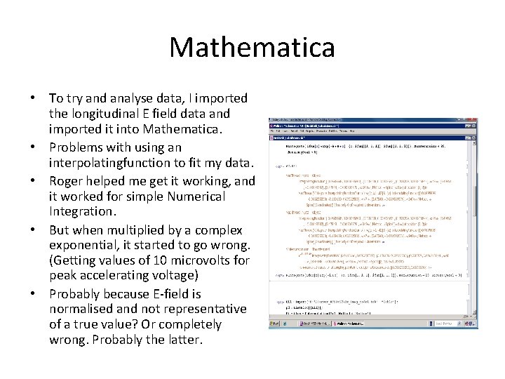
Mathematica • To try and analyse data, I imported the longitudinal E field data and imported it into Mathematica. • Problems with using an interpolatingfunction to fit my data. • Roger helped me get it working, and it worked for simple Numerical Integration. • But when multiplied by a complex exponential, it started to go wrong. (Getting values of 10 microvolts for peak accelerating voltage) • Probably because E-field is normalised and not representative of a true value? Or completely wrong. Probably the latter.

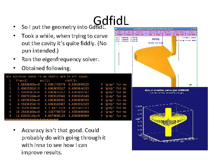
Gdfid. L • So I put the geometry into Gdfid. L. • Took a while, when trying to carve out the cavity it’s quite fiddly. (No pun intended. ) • Ran the eigenfrequency solver. • Obtained following. • Accuracy isn’t that good. Could probably do with going through it with Inna to see how I can improve results.

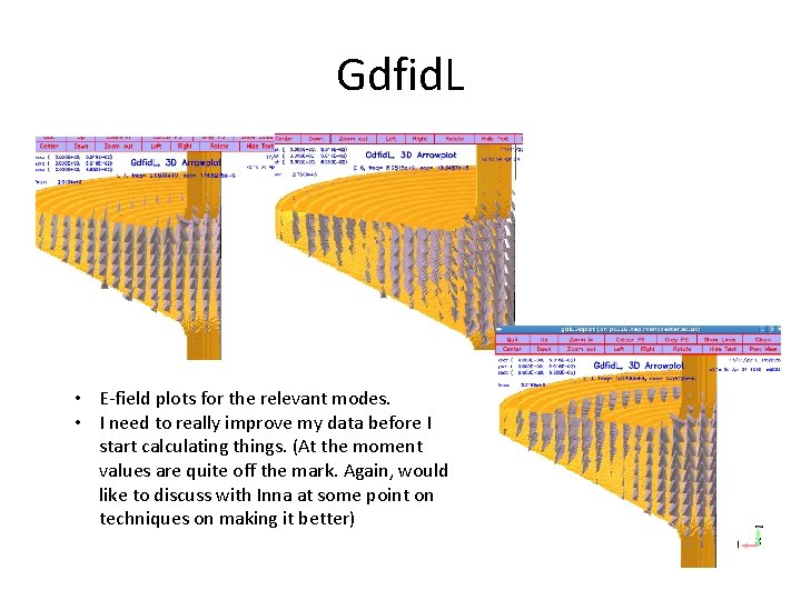
Gdfid. L • E-field plots for the relevant modes. • I need to really improve my data before I start calculating things. (At the moment values are quite off the mark. Again, would like to discuss with Inna at some point on techniques on making it better)