Lecture XIII Galaxy Surveys Part 1 Physics 8803

Lecture XIII: Galaxy Surveys, Part 1 Physics 8803 April 10, 2019 1

Contents • Theory of galaxy clustering • Observational aspects of optical surveys 2

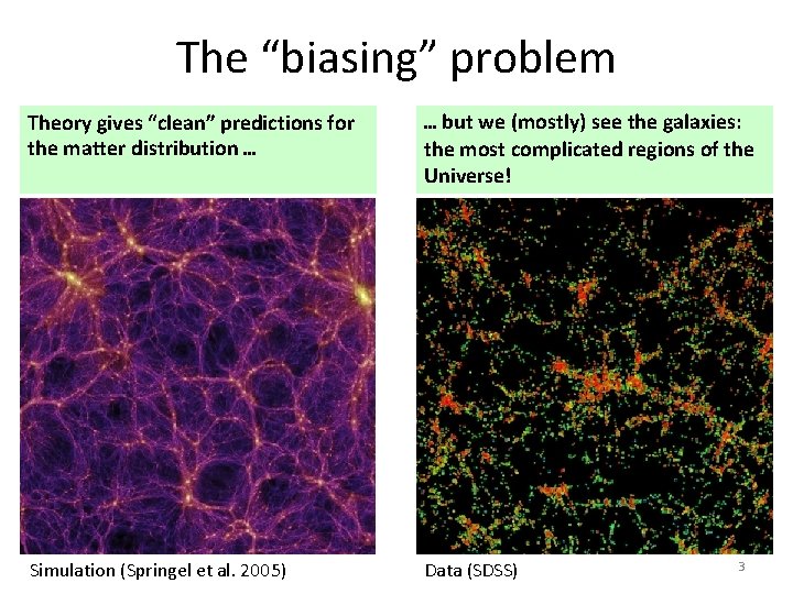
The “biasing” problem Theory gives “clean” predictions for the matter distribution … … but we (mostly) see the galaxies: the most complicated regions of the Universe! Simulation (Springel et al. 2005) Data (SDSS) 3

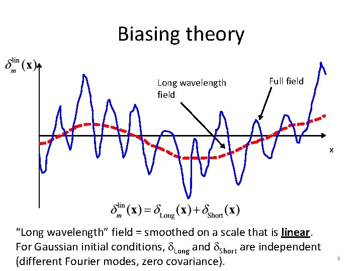
Biasing theory Long wavelength field Full field x “Long wavelength” field = smoothed on a scale that is linear. For Gaussian initial conditions, d. Long and d. Short are independent (different Fourier modes, zero covariance). 4

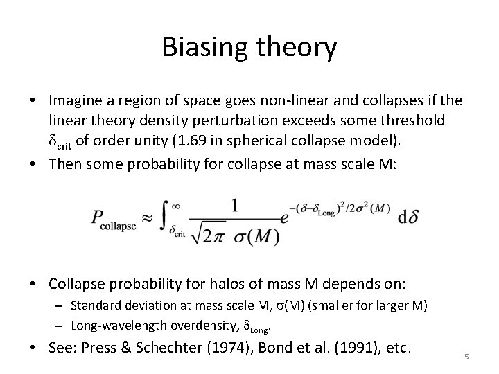
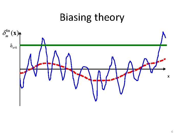
Biasing theory • Imagine a region of space goes non-linear and collapses if the linear theory density perturbation exceeds some threshold dcrit of order unity (1. 69 in spherical collapse model). • Then some probability for collapse at mass scale M: • Collapse probability for halos of mass M depends on: – Standard deviation at mass scale M, s(M) (smaller for larger M) – Long-wavelength overdensity, d. Long. • See: Press & Schechter (1974), Bond et al. (1991), etc. 5

Biasing theory dcrit x 6

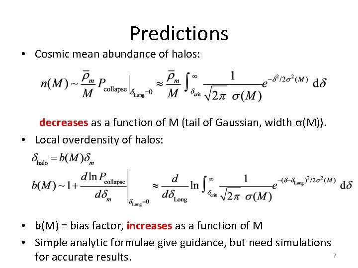
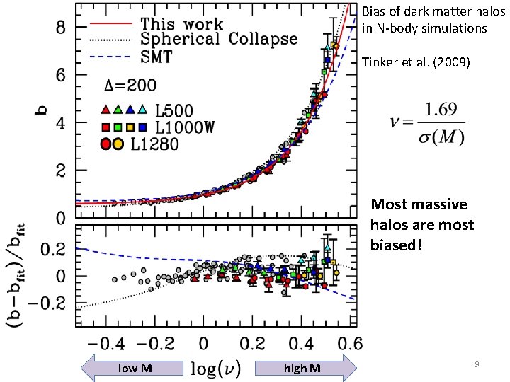
Predictions • Cosmic mean abundance of halos: decreases as a function of M (tail of Gaussian, width s(M)). • Local overdensity of halos: • b(M) = bias factor, increases as a function of M • Simple analytic formulae give guidance, but need simulations 7 for accurate results.

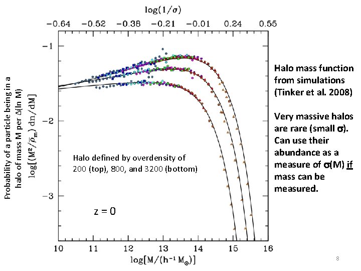
Probability of a particle being in a halo of mass M per ∆(ln M) Halo mass function from simulations (Tinker et al. 2008) Halo defined by overdensity of 200 (top), 800, and 3200 (bottom) Very massive halos are rare (small s). Can use their abundance as a measure of s(M) if mass can be measured. z=0 8

Bias of dark matter halos in N-body simulations Tinker et al. (2009) Most massive halos are most biased! low M high M 9

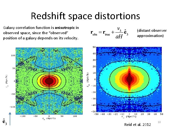
Redshift space distortions Galaxy correlation function is anisotropic in observed space, since the “observed” position of a galaxy depends on its velocity. (distant observer approximation) Reid et al. 2012 10

Observational Aspects • Imaging surveys: – Can go fainter/get more objects in a given amount of telescope time – Colors only, not “real” redshifts (but photo-z’s) – But morphological information (e. g. , shapes for weak lensing) • Spectroscopic surveys: – – Most precise redshifts Spectral diagnostics of galaxies (line widths, ratios of intensities …) But very expensive and sample sizes are smaller (Usually) “target” objects identified in imaging surveys 11

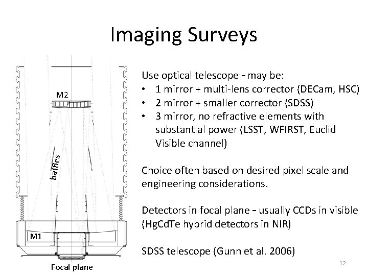
Imaging Surveys baffles M 2 Use optical telescope – may be: • 1 mirror + multi-lens corrector (DECam, HSC) • 2 mirror + smaller corrector (SDSS) • 3 mirror, no refractive elements with substantial power (LSST, WFIRST, Euclid Visible channel) Choice often based on desired pixel scale and engineering considerations. Detectors in focal plane – usually CCDs in visible (Hg. Cd. Te hybrid detectors in NIR) M 1 SDSS telescope (Gunn et al. 2006) Focal plane 12

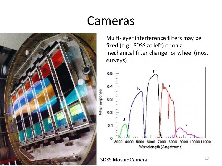
Cameras Multi-layer interference filters may be fixed (e. g. , SDSS at left) or on a mechanical filter changer or wheel (most surveys) r g u SDSS Mosaic Camera i z 13

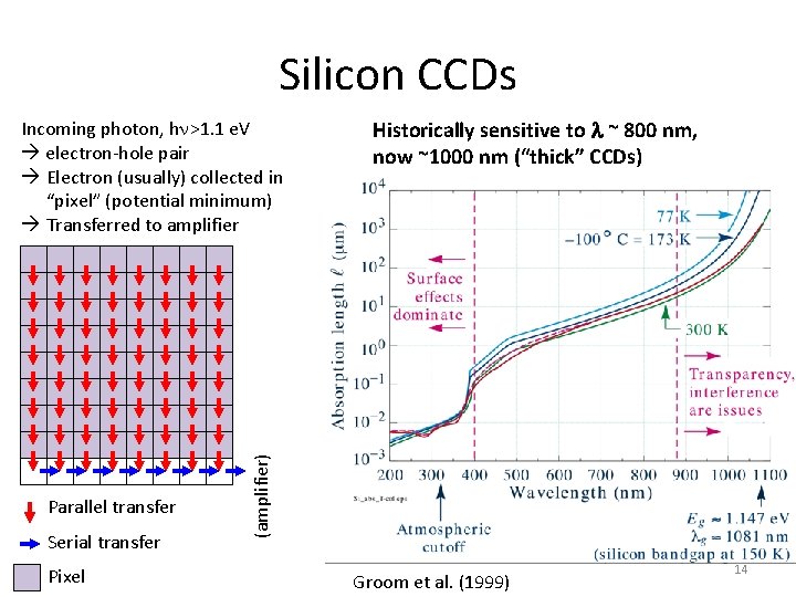
Silicon CCDs Parallel transfer Serial transfer Pixel Historically sensitive to l ~ 800 nm, now ~1000 nm (“thick” CCDs) (amplifier) Incoming photon, hn>1. 1 e. V electron-hole pair Electron (usually) collected in “pixel” (potential minimum) Transferred to amplifier Groom et al. (1999) 14

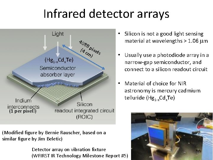
Infrared detector arrays 40 (Hg 1 -x. Cdx. Te) 88 (4 pixel cm s ) • Silicon is not a good light sensing material at wavelengths > 1. 06 mm • Usually use a photodiode array in a narrow-gap semiconductor, and connect to a silicon readout circuit • Material of choice for NIR astronomy is mercury cadmium telluride (Hg 1 -x. Cdx. Te) (1 per pixel!) (Modified figure by Bernie Rauscher, based on a similar figure by Jim Beletic) Detector array on vibration fixture (WFIRST IR Technology Milestone Report #5) 15

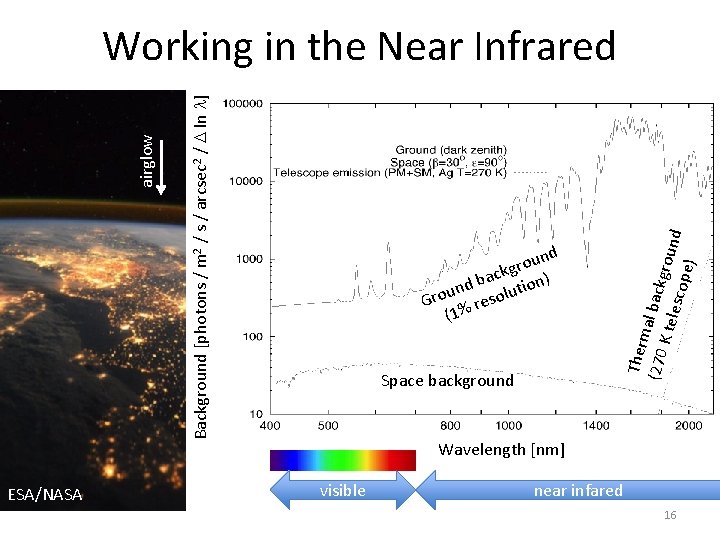
ESA/NASA nd u o r ckg n) a b und solutio o r G re (1% Space background Ther m (270 al backg K tel r esco ound pe) Background [photons / m 2 / s / arcsec 2 / D ln l] airglow Working in the Near Infrared Wavelength [nm] visible near infared 16

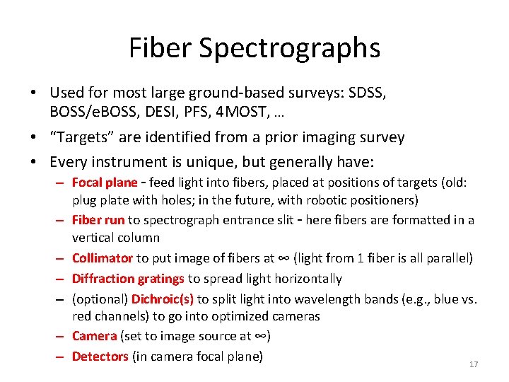
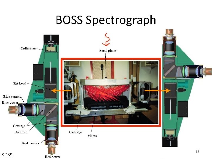
Fiber Spectrographs • Used for most large ground-based surveys: SDSS, BOSS/e. BOSS, DESI, PFS, 4 MOST, … • “Targets” are identified from a prior imaging survey • Every instrument is unique, but generally have: – Focal plane – feed light into fibers, placed at positions of targets (old: plug plate with holes; in the future, with robotic positioners) – Fiber run to spectrograph entrance slit – here fibers are formatted in a vertical column – Collimator to put image of fibers at ∞ (light from 1 fiber is all parallel) – Diffraction gratings to spread light horizontally – (optional) Dichroic(s) to split light into wavelength bands (e. g. , blue vs. red channels) to go into optimized cameras – Camera (set to image source at ∞) – Detectors (in camera focal plane) 17

BOSS Spectrograph SDSS 18

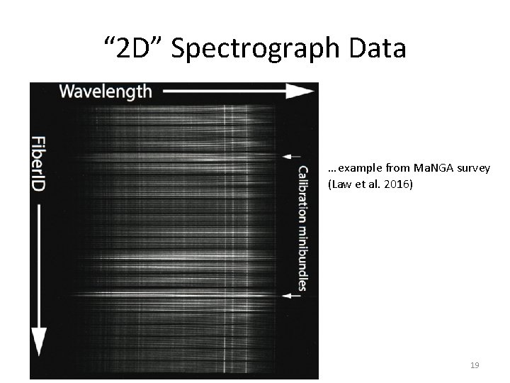
“ 2 D” Spectrograph Data … example from Ma. NGA survey (Law et al. 2016) 19

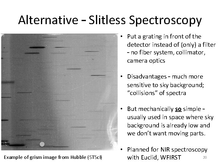
Alternative – Slitless Spectroscopy • Put a grating in front of the detector instead of (only) a filter – no fiber system, collimator, camera optics • Disadvantages – much more sensitive to sky background; “collisions” of spectra • But mechanically so simple – usually used in space where sky background is already low and we don’t want moving parts. Example of grism image from Hubble (STSc. I) • Planned for NIR spectroscopy 20 with Euclid, WFIRST