IP modeling techniques I In this handout Modeling

IP modeling techniques I In this handout, Modeling techniques: ØUsing binary variables ØRestrictions on number of options ØContingent decisions ØVariables (functions) with k possible values Applications: ØFacility Location Problem ØKnapsack Problem

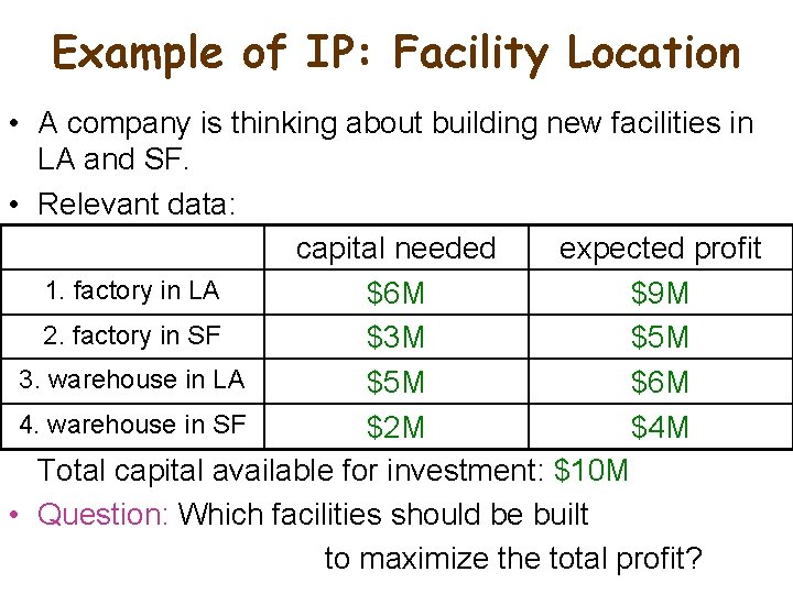
Example of IP: Facility Location • A company is thinking about building new facilities in LA and SF. • Relevant data: capital needed expected profit 1. factory in LA $6 M $9 M 2. factory in SF $3 M $5 M 3. warehouse in LA $5 M $6 M 4. warehouse in SF $2 M $4 M Total capital available for investment: $10 M • Question: Which facilities should be built to maximize the total profit?

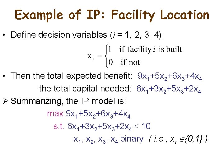
Example of IP: Facility Location • Define decision variables (i = 1, 2, 3, 4): • Then the total expected benefit: 9 x 1+5 x 2+6 x 3+4 x 4 the total capital needed: 6 x 1+3 x 2+5 x 3+2 x 4 Ø Summarizing, the IP model is: max 9 x 1+5 x 2+6 x 3+4 x 4 s. t. 6 x 1+3 x 2+5 x 3+2 x 4 10 x 1, x 2, x 3, x 4 binary ( i. e. , xi {0, 1} )

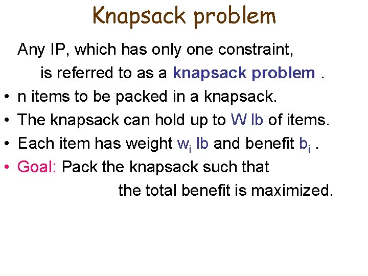
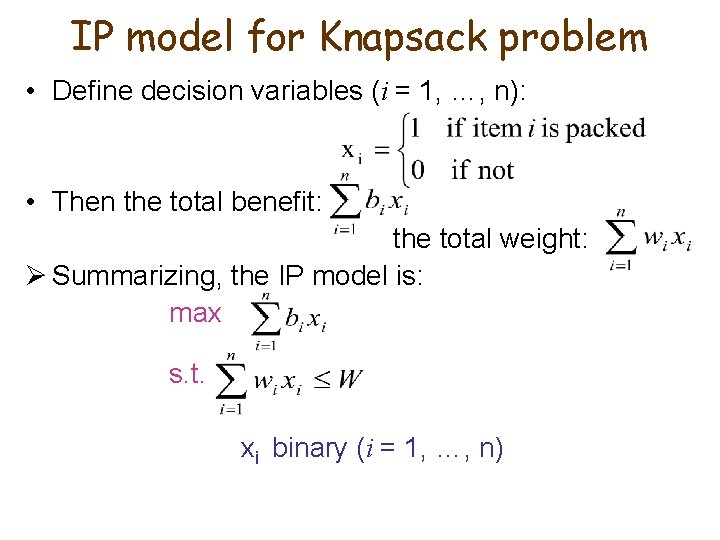
Knapsack problem • • Any IP, which has only one constraint, is referred to as a knapsack problem. n items to be packed in a knapsack. The knapsack can hold up to W lb of items. Each item has weight wi lb and benefit bi. Goal: Pack the knapsack such that the total benefit is maximized.

IP model for Knapsack problem • Define decision variables (i = 1, …, n): • Then the total benefit: the total weight: Ø Summarizing, the IP model is: max s. t. xi binary (i = 1, …, n)

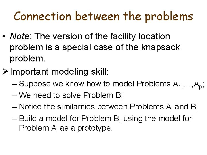
Connection between the problems • Note: The version of the facility location problem is a special case of the knapsack problem. Ø Important modeling skill: – Suppose we know how to model Problems A 1, …, Ap; – We need to solve Problem B; – Notice the similarities between Problems Ai and B; – Build a model for Problem B, using the model for Problem Ai as a prototype.

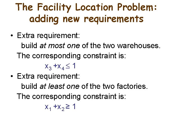
The Facility Location Problem: adding new requirements • Extra requirement: build at most one of the two warehouses. The corresponding constraint is: x 3 +x 4 1 • Extra requirement: build at least one of the two factories. The corresponding constraint is: x 1 +x 2 ≥ 1

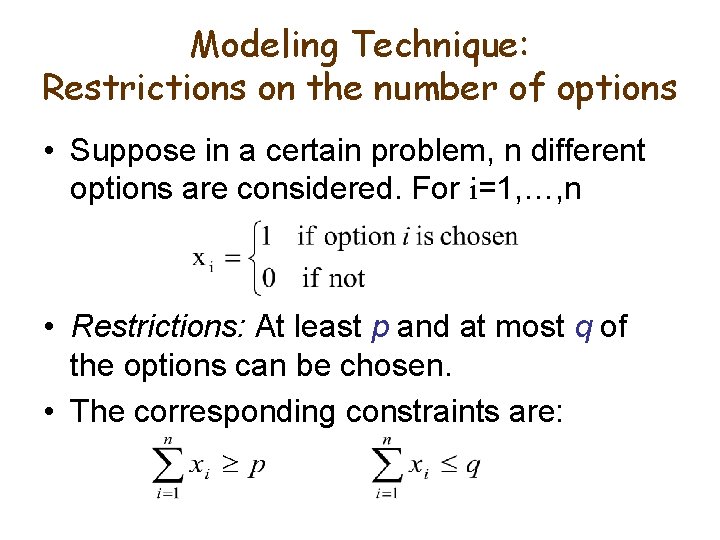
Modeling Technique: Restrictions on the number of options • Suppose in a certain problem, n different options are considered. For i=1, …, n • Restrictions: At least p and at most q of the options can be chosen. • The corresponding constraints are:

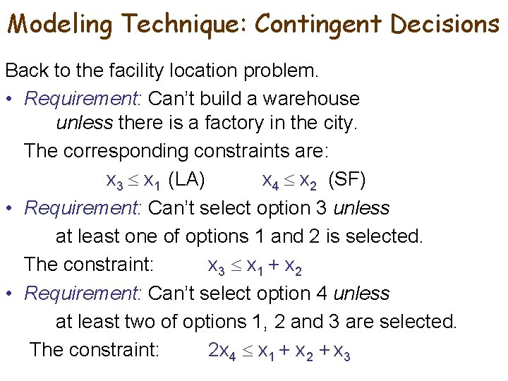
Modeling Technique: Contingent Decisions Back to the facility location problem. • Requirement: Can’t build a warehouse unless there is a factory in the city. The corresponding constraints are: x 3 x 1 (LA) x 4 x 2 (SF) • Requirement: Can’t select option 3 unless at least one of options 1 and 2 is selected. The constraint: x 3 x 1 + x 2 • Requirement: Can’t select option 4 unless at least two of options 1, 2 and 3 are selected. The constraint: 2 x 4 x 1 + x 2 + x 3

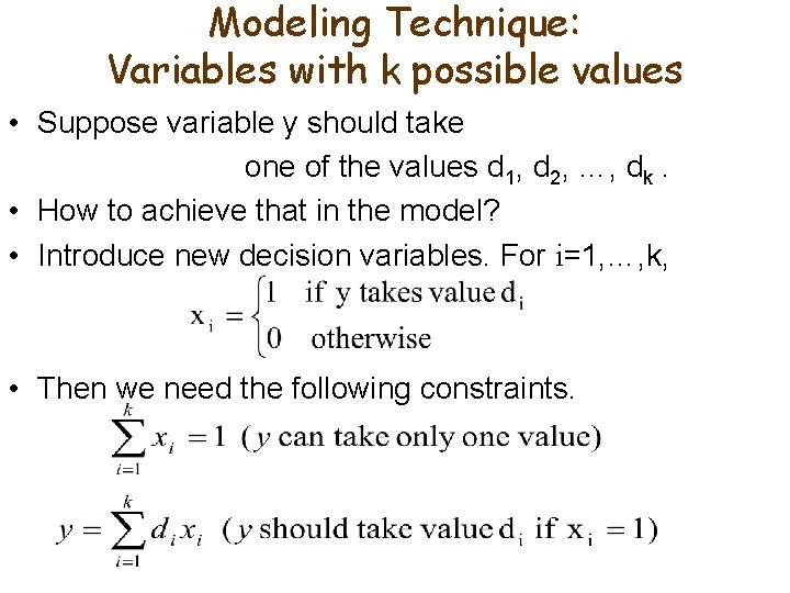
Modeling Technique: Variables with k possible values • Suppose variable y should take one of the values d 1, d 2, …, dk. • How to achieve that in the model? • Introduce new decision variables. For i=1, …, k, • Then we need the following constraints.

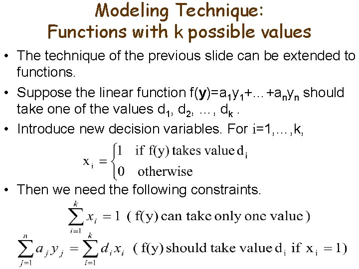
Modeling Technique: Functions with k possible values • The technique of the previous slide can be extended to functions. • Suppose the linear function f(y)=a 1 y 1+…+anyn should take one of the values d 1, d 2, …, dk. • Introduce new decision variables. For i=1, …, k, • Then we need the following constraints.