Introduction to Mapping in SAS Kaeli Samson MA

Introduction to Mapping in SAS Kaeli Samson, MA, MPH University of Nebraska Medical Center Iowa SAS Users Group One-Day Conference May 21 st, 2018

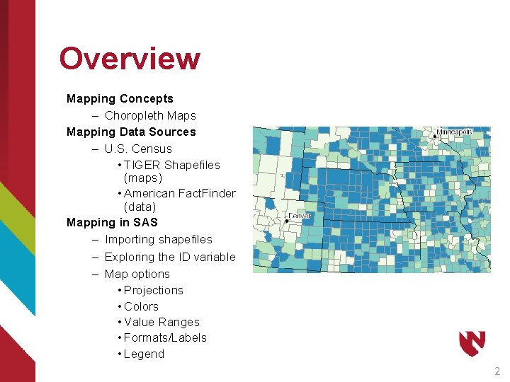
Overview Mapping Concepts – Choropleth Maps Mapping Data Sources – U. S. Census • TIGER Shapefiles (maps) • American Fact. Finder (data) Mapping in SAS – Importing shapefiles – Exploring the ID variable – Map options • Projections • Colors • Value Ranges • Formats/Labels • Legend 2

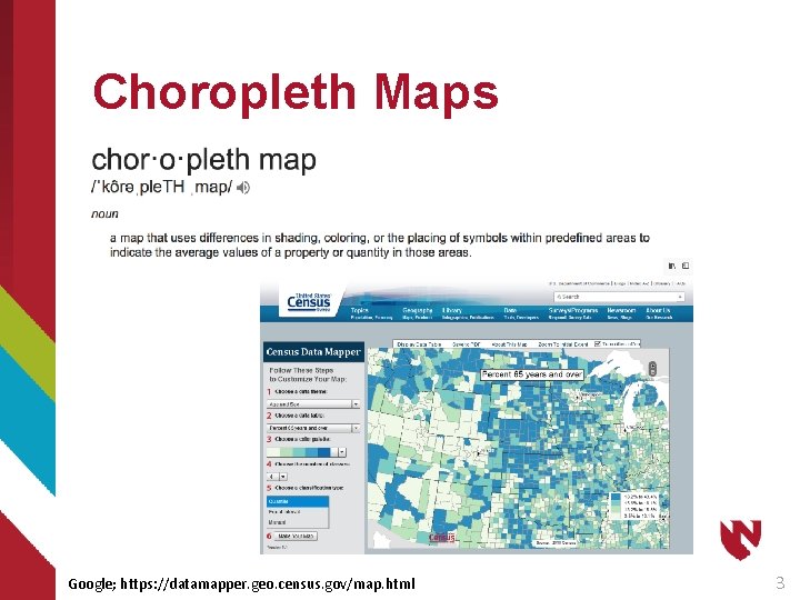
Choropleth Maps Google; https: //datamapper. geo. census. gov/map. html 3

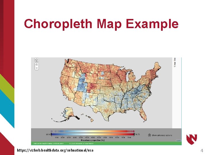
Choropleth Map Example https: //vizhub. healthdata. org/subnational/usa 4

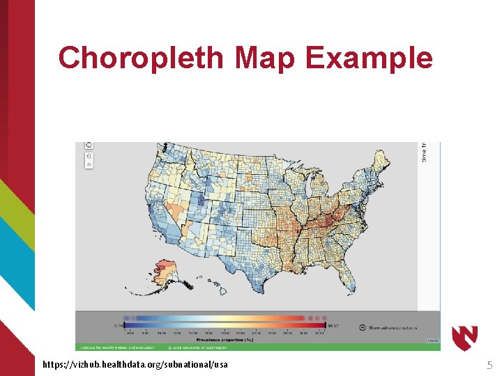
Choropleth Map Example https: //vizhub. healthdata. org/subnational/usa 5

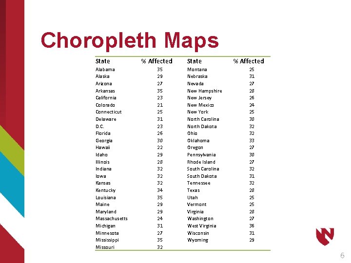
Choropleth Maps State Alabama Alaska Arizona Arkansas California Colorado Connecticut Delaware D. C. Florida Georgia Hawaii Idaho Illinois Indiana Iowa Kansas Kentucky Louisiana Maine Maryland Massachusetts Michigan Minnesota Mississippi Missouri % Affected 35 29 27 35 23 21 25 31 23 26 30 22 29 28 32 32 32 34 35 29 29 24 31 27 35 32 State Montana Nebraska Nevada New Hampshire New Jersey New Mexico New York North Carolina North Dakota Ohio Oklahoma Oregon Pennsylvania Rhode Island South Carolina South Dakota Tennessee Texas Utah Vermont Virginia Washington West Virginia Wisconsin Wyoming % Affected 25 31 27 28 26 24 25 30 32 32 33 27 30 27 32 31 32 28 25 25 28 27 36 31 29 6

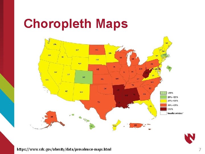
Choropleth Maps https: //www. cdc. gov/obesity/data/prevalence-maps. html 7

Using SAS to Make Maps 8

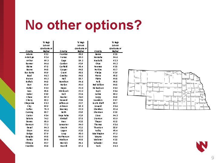
No other options? County Adams Antelope Arthur Banner Blaine Boone Box Butte Boyd Brown Buffalo Burt Butler Cass Cedar Chase Cherry Cheyenne Clay Colfax Cuming Custer Dakota Dawes Dawson Deuel Dixon Dodge Douglas Dundy Fillmore Franklin % High School Graduate or Higher 92. 1 92. 6 99. 3 94. 6 97. 8 94. 5 90. 9 96. 2 90. 2 94. 8 91. 9 92. 0 95. 5 93. 9 89. 3 88. 1 93. 2 89. 9 75. 3 88. 7 93. 4 74. 1 95. 0 77. 1 94. 3 90. 6 87. 9 90. 5 89. 5 90. 7 90. 8 County Frontier Furnas Gage Garden Garfield Gosper Grant Greeley Hall Hamilton Harlan Hayes Hitchcock Holt Hooker Howard Jefferson Johnson Kearney Keith Keya Paha Kimball Knox Lancaster Lincoln Logan Loup Mc. Pherson Madison Merrick Morrill % High School Graduate or Higher 95. 8 89. 0 89. 2 93. 9 95. 4 94. 8 95. 5 94. 5 85. 7 94. 6 90. 0 92. 3 92. 2 92. 4 96. 0 93. 5 92. 7 89. 3 92. 3 93. 9 92. 9 87. 5 92. 8 94. 0 92. 1 92. 8 98. 0 91. 0 90. 5 95. 1 87. 1 County Nance Nemaha Nuckolls Otoe Pawnee Perkins Phelps Pierce Platte Polk Red Willow Richardson Rock Saline Sarpy Saunders Scotts Bluff Seward Sheridan Sherman Sioux Stanton Thayer Thomas Thurston Valley Washington Wayne Webster Wheeler York % High School Graduate or Higher 92. 5 94. 6 92. 3 90. 2 92. 5 91. 7 92. 9 95. 8 90. 5 95. 5 94. 5 93. 0 93. 4 88. 1 94. 8 93. 7 88. 7 93. 6 91. 6 92. 8 94. 3 91. 0 91. 8 93. 6 88. 9 95. 4 97. 1 96. 4 92. 8 94. 8 93. 3 9

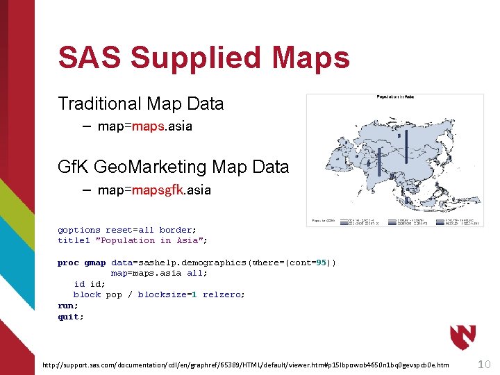
SAS Supplied Maps Traditional Map Data – map=maps. asia Gf. K Geo. Marketing Map Data – map=mapsgfk. asia goptions reset=all border; title 1 "Population in Asia"; proc gmap data=sashelp. demographics(where=(cont=95)) map=maps. asia all; id id; block pop / blocksize=1 relzero; run; quit; http: //support. sas. com/documentation/cdl/en/graphref/65389/HTML/default/viewer. htm#p 15 lbpowob 4650 n 1 bq 0 gevspcb 0 e. htm 10

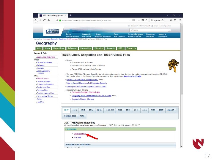
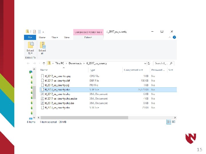
U. S. Census: Shapefiles 1

12

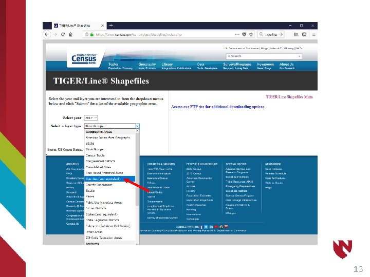
13

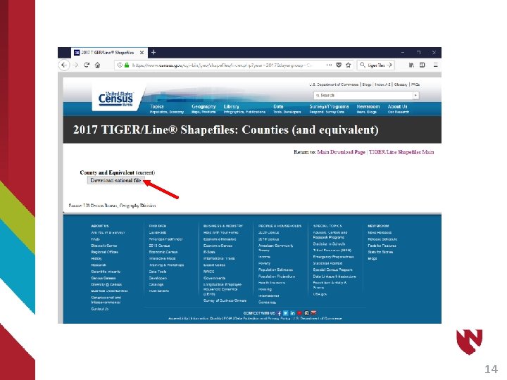
14

15

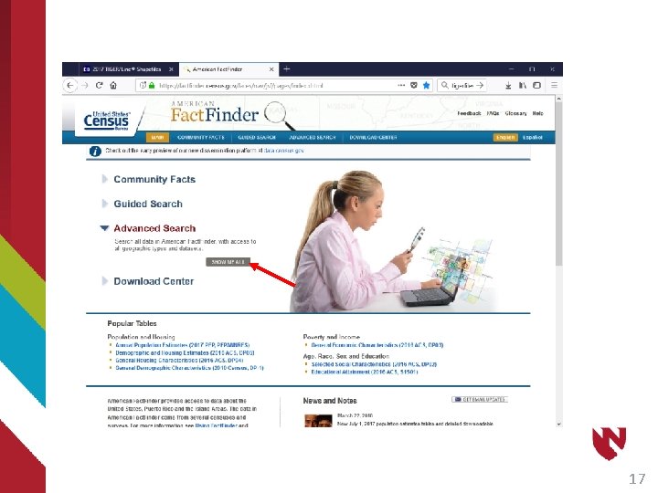
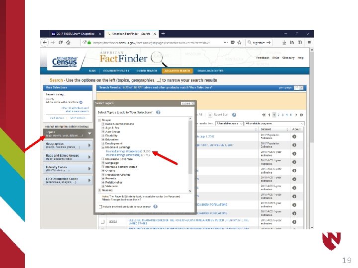
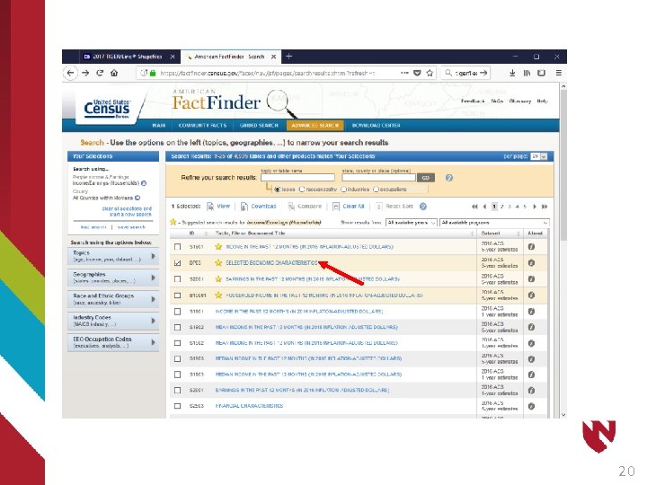
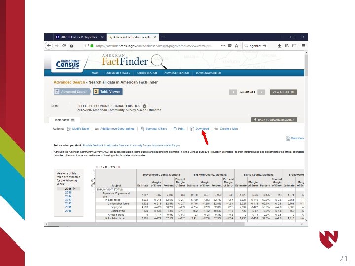
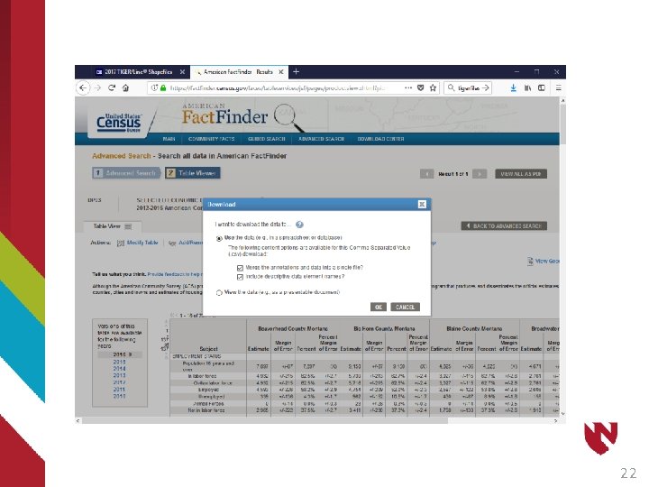
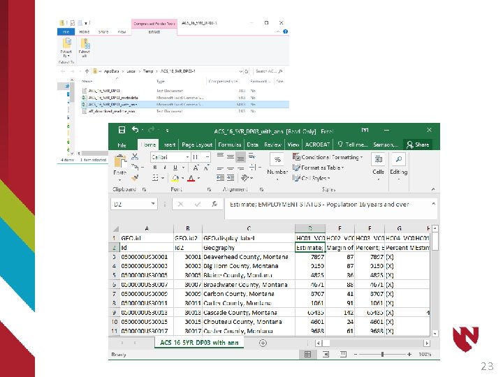
U. S. Census: Data 16

17

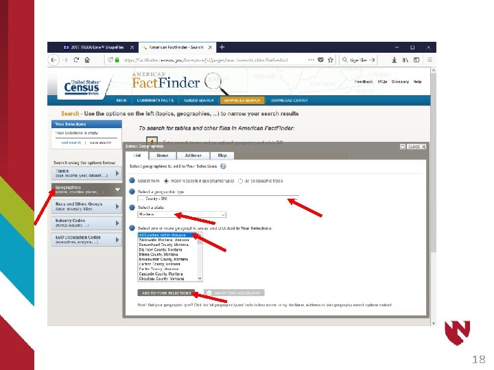
18

19

20

21

22

23

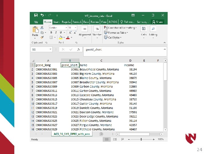
24

Making Maps in SAS 25

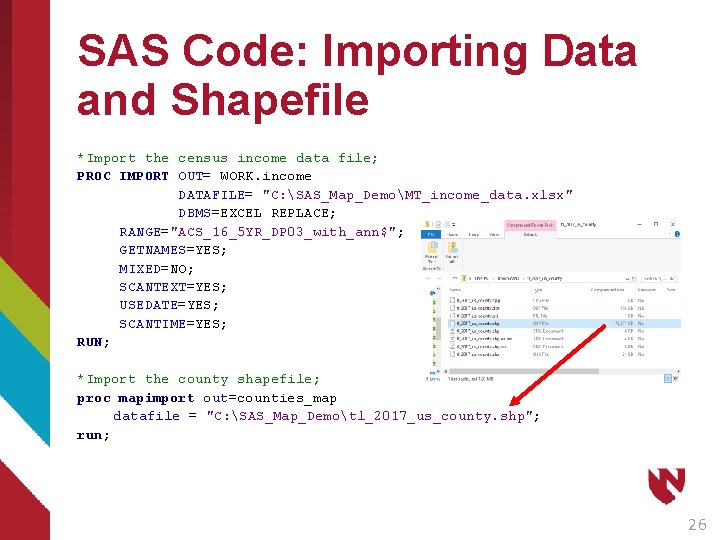
SAS Code: Importing Data and Shapefile *Import the census income data file; PROC IMPORT OUT= WORK. income DATAFILE= "C: SAS_Map_DemoMT_income_data. xlsx" DBMS=EXCEL REPLACE; RANGE="ACS_16_5 YR_DP 03_with_ann$"; GETNAMES=YES; MIXED=NO; SCANTEXT=YES; USEDATE=YES; SCANTIME=YES; RUN; *Import the county shapefile; proc mapimport out=counties_map datafile = "C: SAS_Map_Demotl_2017_us_county. shp"; run; 26

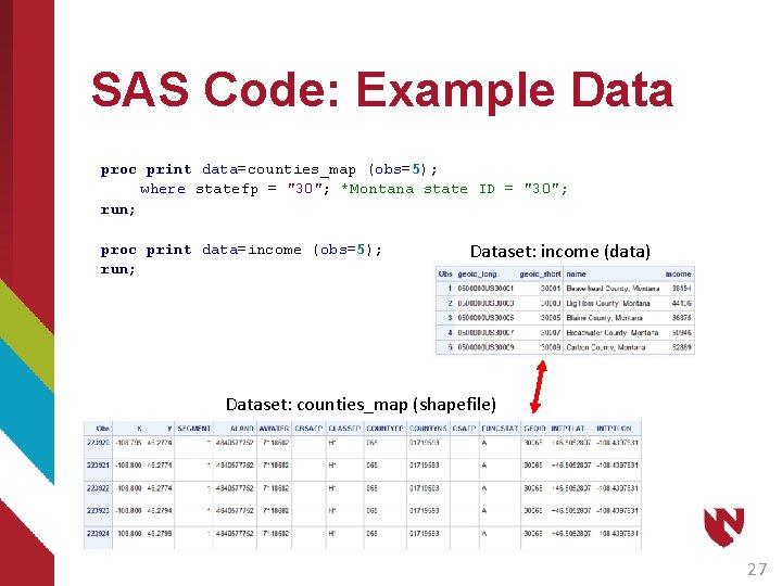
SAS Code: Example Data proc print data=counties_map (obs=5); where statefp = "30"; *Montana state ID = "30"; run; proc print data=income (obs=5); run; Dataset: income (data) Dataset: counties_map (shapefile) 27

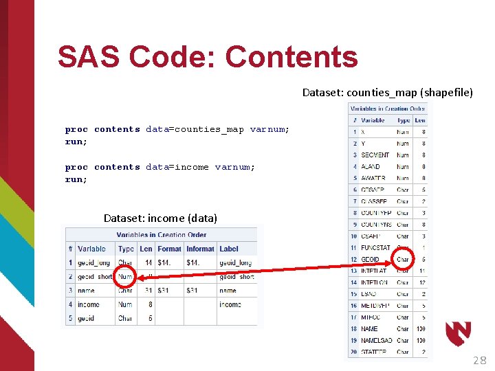
SAS Code: Contents Dataset: counties_map (shapefile) proc contents data=counties_map varnum; run; proc contents data=income varnum; run; Dataset: income (data) 28

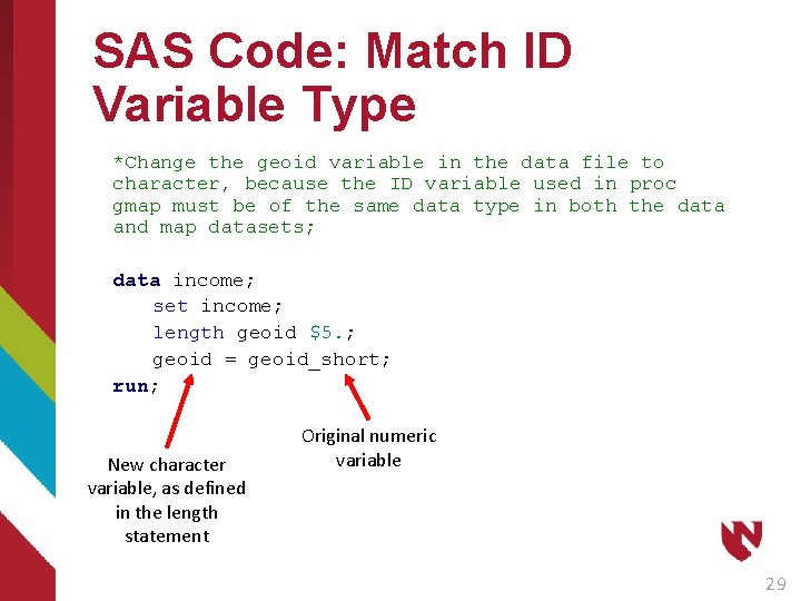
SAS Code: Match ID Variable Type *Change the geoid variable in the data file to character, because the ID variable used in proc gmap must be of the same data type in both the data and map datasets; data income; set income; length geoid $5. ; geoid = geoid_short; run; New character variable, as defined in the length statement Original numeric variable 29

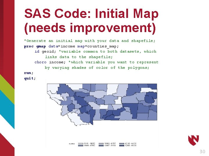
SAS Code: Initial Map (needs improvement) *Generate an initial map with your data and shapefile; proc gmap data=income map=counties_map; id geoid; *variable common to both datasets, which links data to the shapefile; choro income; *which variable you want to represent by varying shades of color of the polygons; run; quit; 30

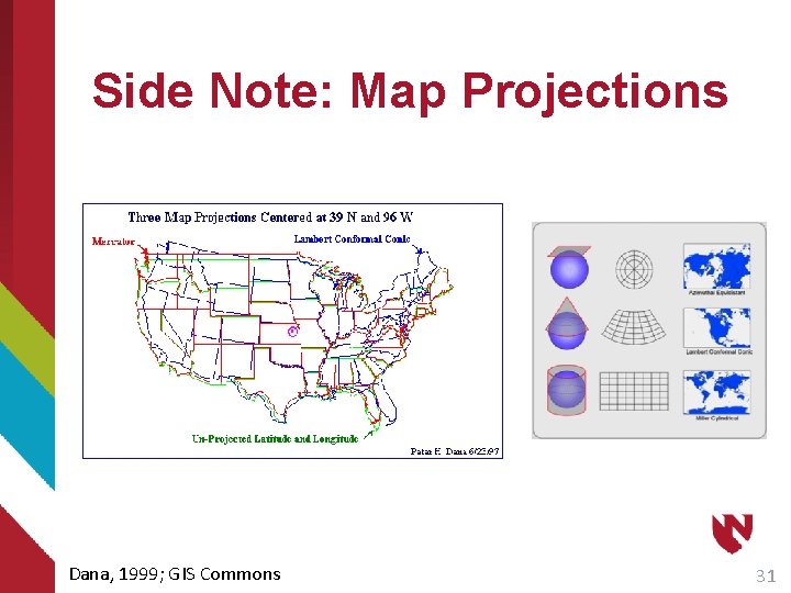
Side Note: Map Projections Dana, 1999; GIS Commons 31

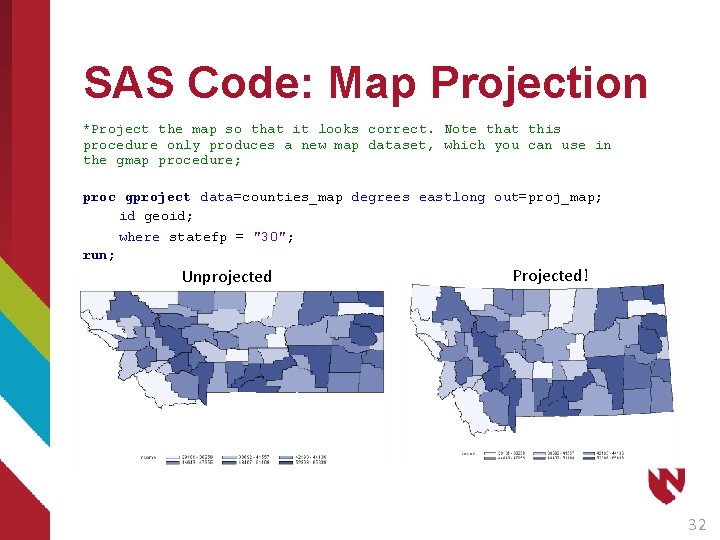
SAS Code: Map Projection *Project the map so that it looks correct. Note that this procedure only produces a new map dataset, which you can use in the gmap procedure; proc gproject data=counties_map degrees eastlong out=proj_map; id geoid; where statefp = "30"; run; Unprojected Projected! 32

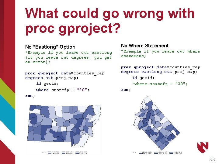
What could go wrong with proc gproject? No “Eastlong” Option *Example if you leave out eastlong (if you leave out degrees, you get an error); proc gproject data=counties_map degrees out=proj_map; id geoid; where statefp = "30"; run; No Where Statement *Example if you leave out where statement; proc gproject data=counties_map degrees eastlong out=proj_map; id geoid; *where statefp = "30"; run; 33

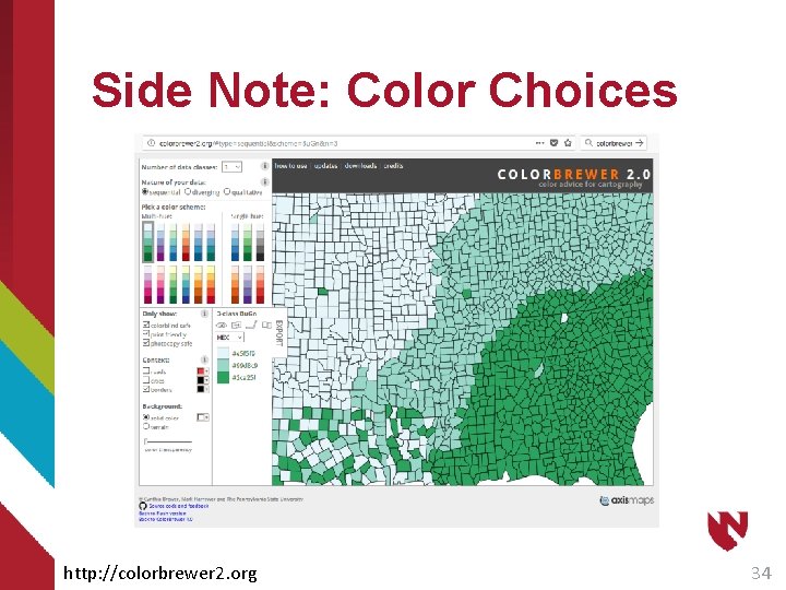
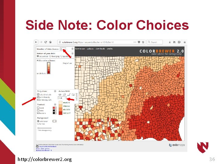
Side Note: Color Choices http: //colorbrewer 2. org 34

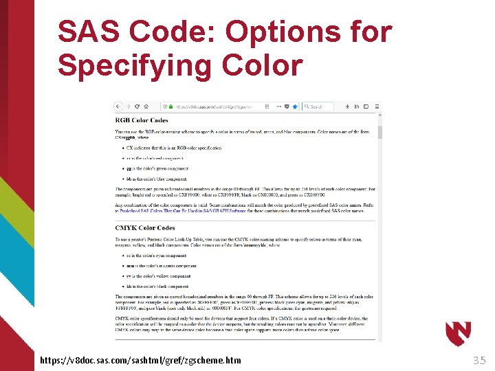
SAS Code: Options for Specifying Color https: //v 8 doc. sas. com/sashtml/gref/zgscheme. htm 35

Side Note: Color Choices http: //colorbrewer 2. org 36

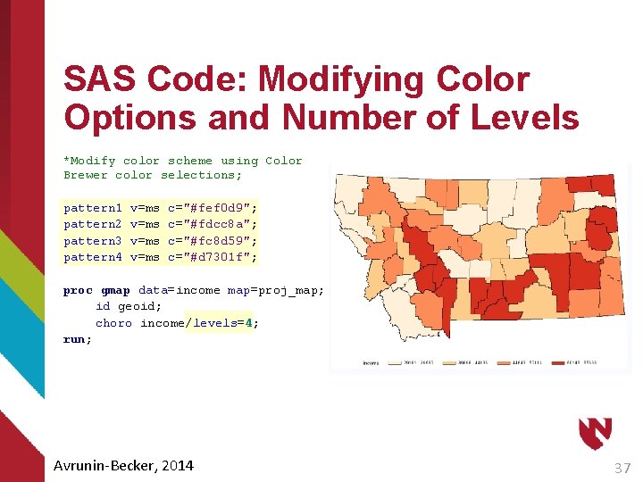
SAS Code: Modifying Color Options and Number of Levels *Modify color scheme using Color Brewer color selections; pattern 1 pattern 2 pattern 3 pattern 4 v=ms c="#fef 0 d 9"; c="#fdcc 8 a"; c="#fc 8 d 59"; c="#d 7301 f"; proc gmap data=income map=proj_map; id geoid; choro income/levels=4; run; Avrunin-Becker, 2014 37

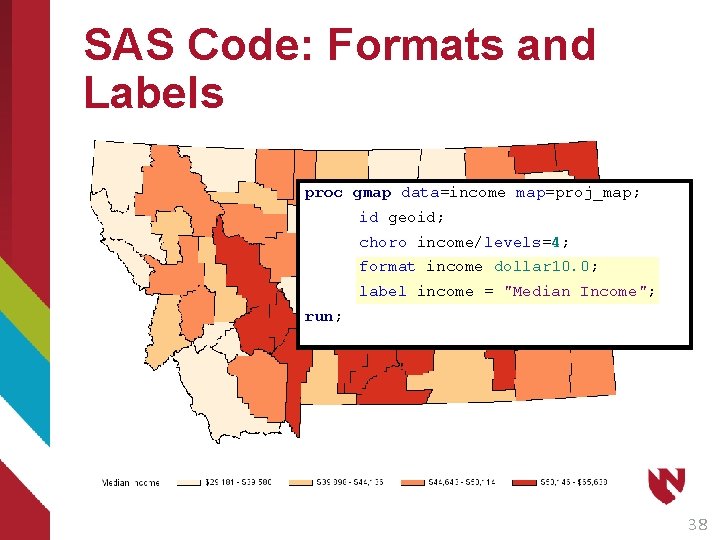
SAS Code: Formats and Labels proc gmap data=income map=proj_map; id geoid; choro income/levels=4; format income dollar 10. 0; label income = "Median Income"; run; 38

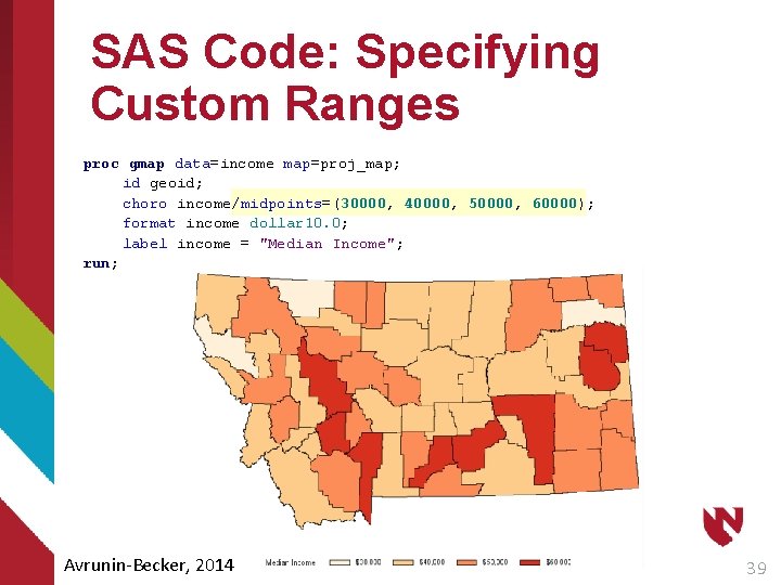
SAS Code: Specifying Custom Ranges proc gmap data=income map=proj_map; id geoid; choro income/midpoints=(30000, 40000, 50000, 60000); format income dollar 10. 0; label income = "Median Income"; run; Avrunin-Becker, 2014 39

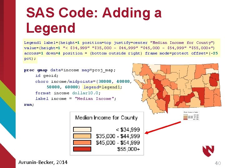
SAS Code: Adding a Legend 1 label=(height=1 position=top justify=center "Median Income for County") value=(height=1 "< $34, 999" "$35, 000 - $44, 999" "$45, 000 - $54, 999" "$55, 000+") across=1 down=4 position = (bottom outside right) frame mode=protect offset=(-25 pct); proc gmap data=income map=proj_map; id geoid; choro income/midpoints=(30000, 40000, 50000, 60000) legend=legend 1; format income dollar 10. 0; label income = "Median Income"; run; Avrunin-Becker, 2014 40

References (those not already presented on slides) • Avrunin-Becker, S. , 2014. How to Make an Impressive Map of the United States with SAS/Graph® for Beginners. SESUG 2014. Retrieved from: https: //analytics. ncsu. edu/sesug/2014/RIV-13. pdf • Dana, P. H. The Geographer's Craft Project, Department of Geography, The University of Colorado at Boulder. Retrieved from: https: //www. colorado. edu/geography/gcraft/notes/mapproj/mappr oj_f. html • GIS Commons. Retrieved from: http: //giscommons. org/earth-andmap-preprocessing/ • Zdeb, M. , 2011. From Shapefiles to Maps Via PROC MAPIMPORT and PROC GMAP. NESUG 2011: Graphics and Reporting. Retrieved from: https: //www. lexjansen. com/nesug 11/gr/gr 11. pdf 41

Questions?