Human Genetics Concepts and Applications Twelfth Edition Chapter

Human Genetics Concepts and Applications Twelfth Edition Chapter 14 Constant Allele Frequencies and DNA Forensics © Mc. Graw-Hill Education. All rights reserved. Authorized only for instructor use in the classroom. No reproduction or further distribution permitted without the prior written consent of Mc. Graw-Hill Education.

Chapter 3 Learning Outcomes (1 of 2) 1. State the unit of information of genetics at the population level. 2. Define gene pool. 3. List the five processes that cause microevolutionary change. 4. State the consequence of macroevolutionary change. 5. State the genotypes represented in each part of the Hardy-Weinberg equation. © Mc. Graw-Hill Education. 14 -2

Chapter 3 Learning Outcomes (2 of 2) 6. Explain the conditions necessary for Hardy. Weinberg equilibrium. 7. Explain how the Hardy-Weinberg equilibrium uses population incidence statistics to predict the probability of a particular phenotype. 8. Explain how parts of the genome that are in Hardy-Weinberg equilibrium can be used to identify individuals. © Mc. Graw-Hill Education. 14 -3

Chapter 3 Introduction Population: Interbreeding group of the same species in a given geographical area Gene pool: Collection of alleles in the members of the population Population genetics: Study of the genetics of a population and how the alleles vary with time Gene Flow: Movement of alleles between populations when people migrate and mate © Mc. Graw-Hill Education. 14 -4

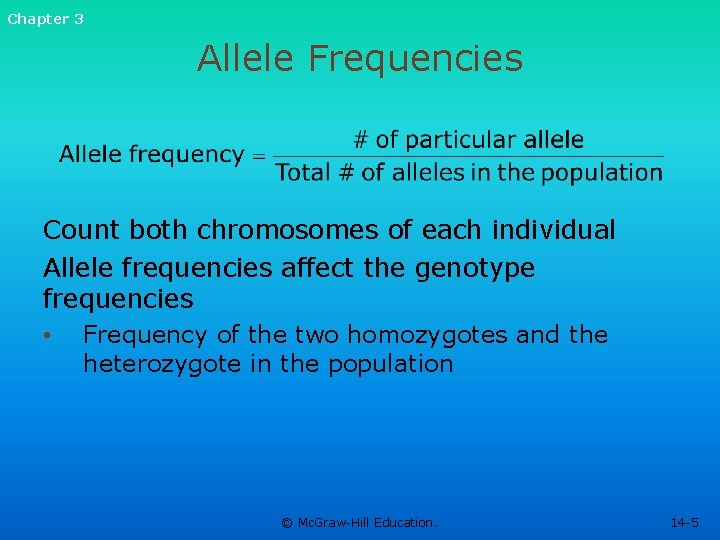
Chapter 3 Allele Frequencies Count both chromosomes of each individual Allele frequencies affect the genotype frequencies • Frequency of the two homozygotes and the heterozygote in the population © Mc. Graw-Hill Education. 14 -5

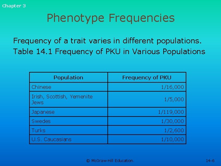
Chapter 3 Phenotype Frequencies Frequency of a trait varies in different populations. Table 14. 1 Frequency of PKU in Various Population Frequency of PKU Chinese 1/16, 000 Irish, Scottish, Yemenite Jews Japanese 1/5, 000 1/119, 000 Swedes 1/30, 000 Turks 1/2, 600 U. S. Caucasians 1/10, 000 © Mc. Graw-Hill Education. 14 -6

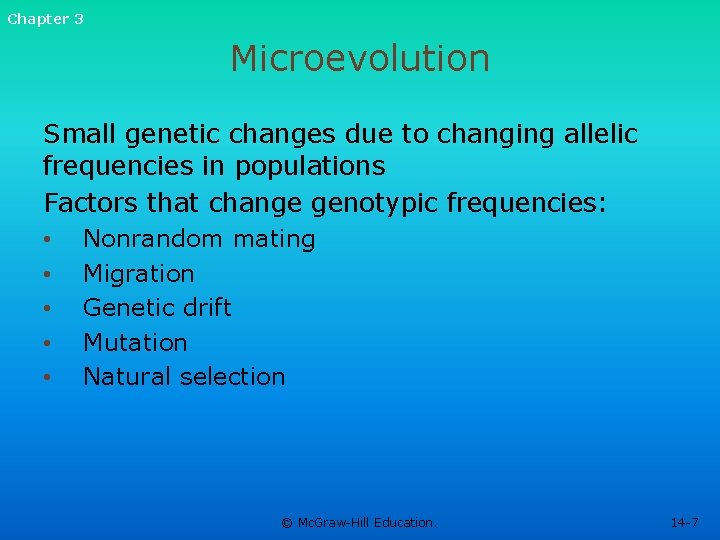
Chapter 3 Microevolution Small genetic changes due to changing allelic frequencies in populations Factors that change genotypic frequencies: • • • Nonrandom mating Migration Genetic drift Mutation Natural selection © Mc. Graw-Hill Education. 14 -7

Chapter 3 Macroevolution Formation of new species Occurs when enough microevolutionary changes have occurred to prevent individuals from one population to successfully produce fertile offspring © Mc. Graw-Hill Education. 14 -8

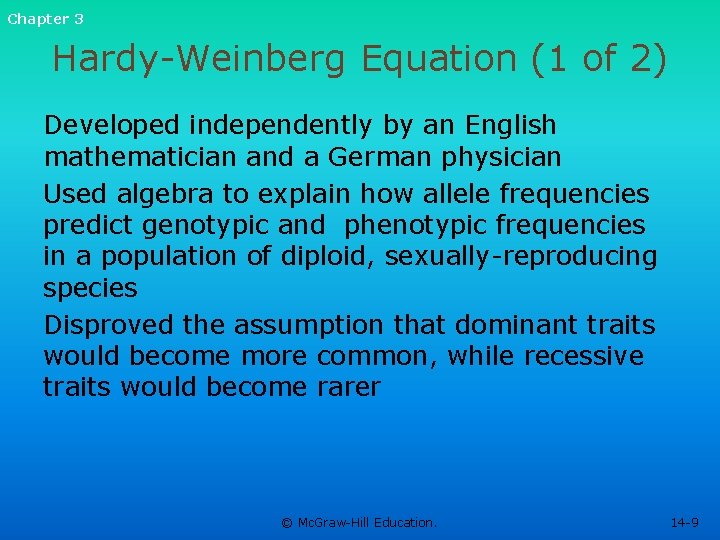
Chapter 3 Hardy-Weinberg Equation (1 of 2) Developed independently by an English mathematician and a German physician Used algebra to explain how allele frequencies predict genotypic and phenotypic frequencies in a population of diploid, sexually-reproducing species Disproved the assumption that dominant traits would become more common, while recessive traits would become rarer © Mc. Graw-Hill Education. 14 -9

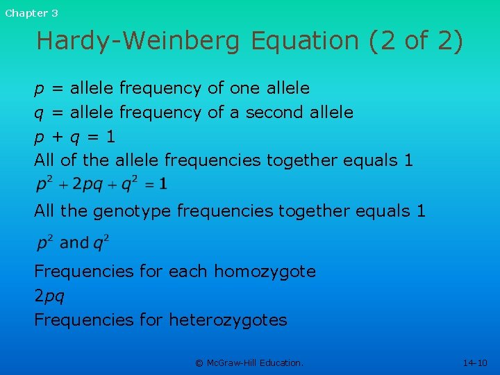
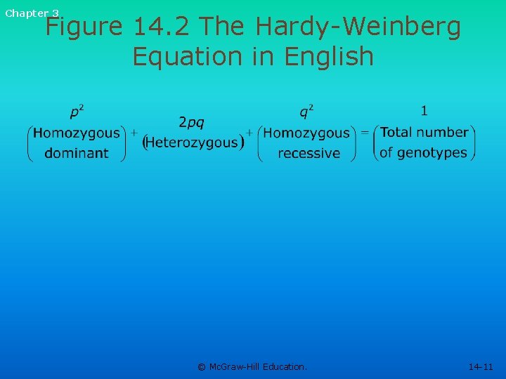
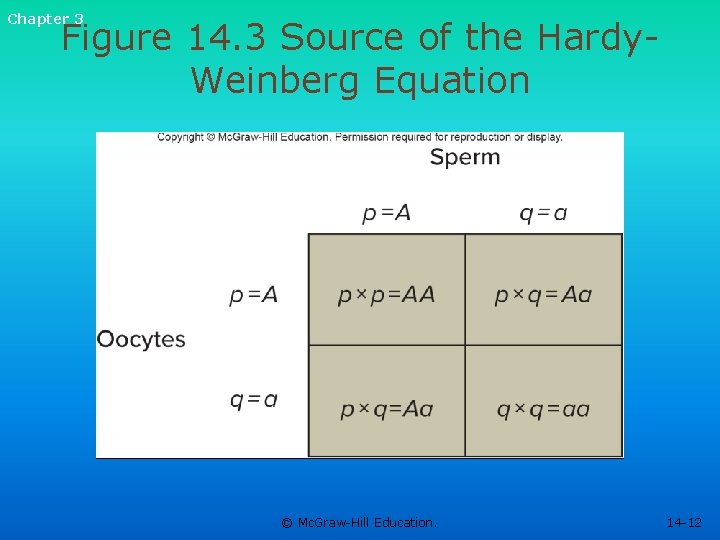
Chapter 3 Hardy-Weinberg Equation (2 of 2) p = allele frequency of one allele q = allele frequency of a second allele p+q=1 All of the allele frequencies together equals 1 All the genotype frequencies together equals 1 Frequencies for each homozygote 2 pq Frequencies for heterozygotes © Mc. Graw-Hill Education. 14 -10

Chapter 3 Figure 14. 2 The Hardy-Weinberg Equation in English © Mc. Graw-Hill Education. 14 -11

Chapter 3 Figure 14. 3 Source of the Hardy. Weinberg Equation © Mc. Graw-Hill Education. 14 -12

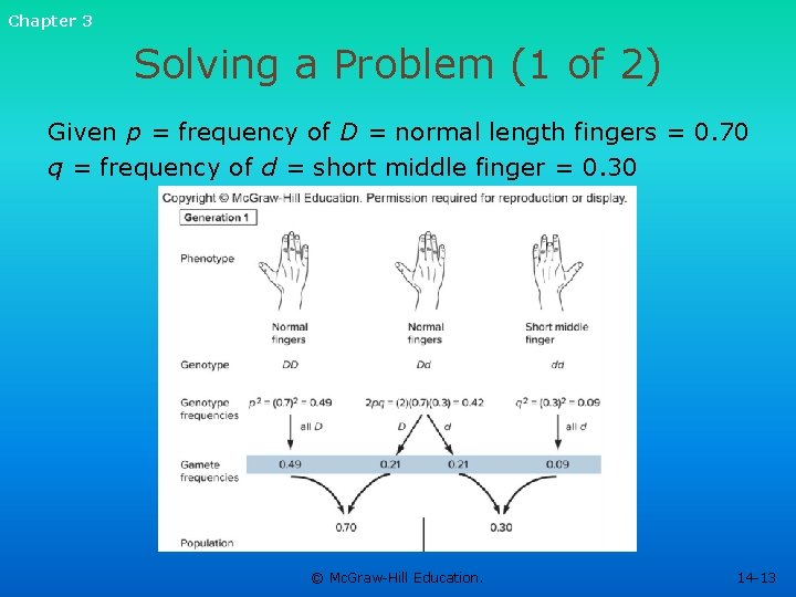
Chapter 3 Solving a Problem (1 of 2) Given p = frequency of D = normal length fingers = 0. 70 q = frequency of d = short middle finger = 0. 30 © Mc. Graw-Hill Education. 14 -13

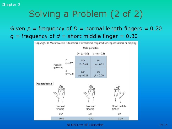
Chapter 3 Solving a Problem (2 of 2) Given p = frequency of D = normal length fingers = 0. 70 q = frequency of d = short middle finger = 0. 30 © Mc. Graw-Hill Education. 14 -14

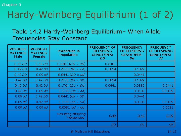
Chapter 3 Hardy-Weinberg Equilibrium (1 of 2) Table 14. 2 Hardy-Weinberg Equilibrium– When Allele Frequencies Stay Constant FREQUENCY OF OFFSPRNG GENOTYPES: DD FREQUENCY OF OFFSPRNG GENOTYPES: Dd FREQUENCY OF OFFSPRNG GENOTYPES: dd POSSIBLE MATINGS: Male POSSIBLE MATINGS: Female 0. 49 DD 0. 2401 (DD × DD) 0. 2401 0. 49 DD 0. 42 Dd 0. 2058 (DD × Dd) 0. 1029 0. 49 DD 0. 09 dd 0. 0441 (DD × dd) 0. 42 Dd 0. 49 DD 0. 2058 (Dd × DD) 0. 1029 0. 42 Dd 0. 1764 (Dd × Dd) 0. 0441 0. 0882 0. 0441 0. 42 Dd 0. 09 dd 0. 0378 (Dd × dd) 0. 0189 0. 09 dd 0. 42 DD 0. 0441 (dd × DD) 0. 0441 0. 09 dd 0. 42 Dd 0. 0378 (dd × Dd) 0. 0189 0. 09 dd 0. 0081 (dd × dd) Proportion in Population Resulting offspring frequencies: 0. 1029 0. 0441 0. 0189 0. 0081 0. 49 0. 42 0. 09 DD Dd dd © Mc. Graw-Hill Education. 14 -15

Chapter 3 Hardy-Weinberg Equilibrium (2 of 2) Allele and genotypic frequencies do not change from one generation to the next. Gene is in Hardy-Weinberg equilibrium. Rare for protein-encoding genes that affect the phenotype Applies to portions of the genome that do not affect phenotype Includes repeated DNA segments • Not subject to natural selection © Mc. Graw-Hill Education. 14 -16

Chapter 3 Applying the Hardy-Weinberg Equation Used to determine carrier probability For autosomal recessive diseases, the homozygous recessive class is used to determine the frequency of alleles in a population • Phenotype indicates its genotype © Mc. Graw-Hill Education. 14 -17

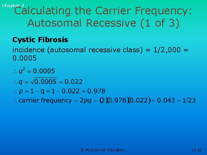
Chapter 3 Calculating the Carrier Frequency: Autosomal Recessive (1 of 3) Cystic Fibrosis incidence (autosomal recessive class) = 1/2, 000 = 0. 0005 © Mc. Graw-Hill Education. 14 -18

Chapter 3 Calculating the Carrier Frequency: Autosomal Recessive (2 of 3) Table 14. 3 Carrier Frequency for Cystic Fibrosis Population Group Carrier Frequency African Americans 1 in 66 Asian Americans 1 in 150 Caucasians of European descent 1 in 23 Hispanic Americans 1 in 46 © Mc. Graw-Hill Education. 14 -19

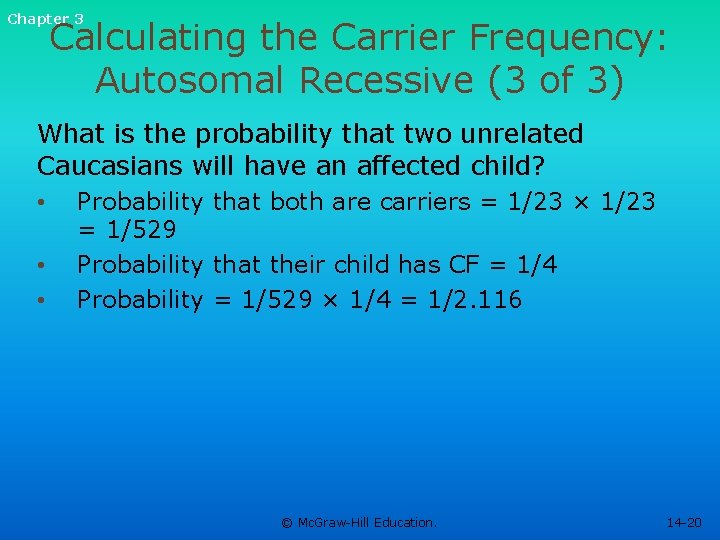
Chapter 3 Calculating the Carrier Frequency: Autosomal Recessive (3 of 3) What is the probability that two unrelated Caucasians will have an affected child? • • • Probability that both are carriers = 1/23 × 1/23 = 1/529 Probability that their child has CF = 1/4 Probability = 1/529 × 1/4 = 1/2. 116 © Mc. Graw-Hill Education. 14 -20

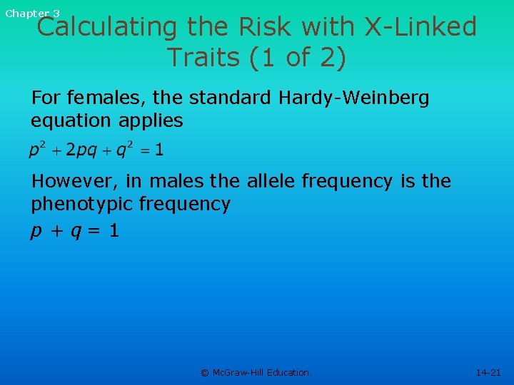
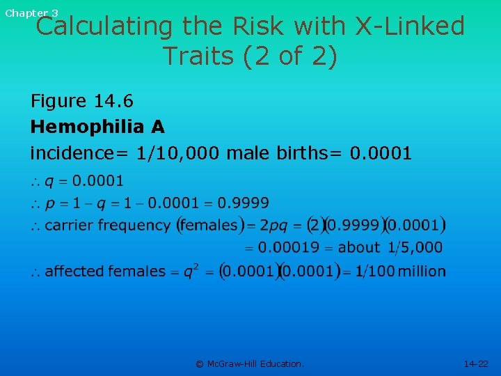
Chapter 3 Calculating the Risk with X-Linked Traits (1 of 2) For females, the standard Hardy-Weinberg equation applies However, in males the allele frequency is the phenotypic frequency p + q= 1 © Mc. Graw-Hill Education. 14 -21

Chapter 3 Calculating the Risk with X-Linked Traits (2 of 2) Figure 14. 6 Hemophilia A incidence= 1/10, 000 male births= 0. 0001 © Mc. Graw-Hill Education. 14 -22

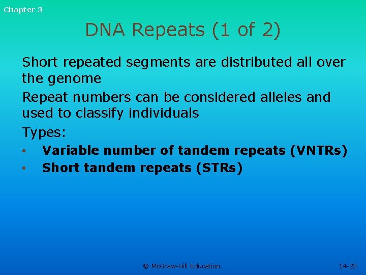
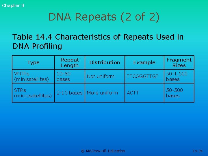
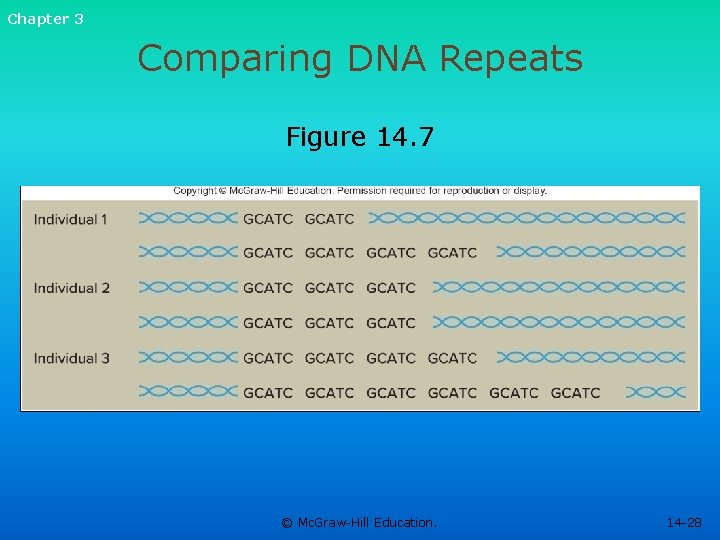
Chapter 3 DNA Repeats (1 of 2) Short repeated segments are distributed all over the genome Repeat numbers can be considered alleles and used to classify individuals Types: • • Variable number of tandem repeats (VNTRs) Short tandem repeats (STRs) © Mc. Graw-Hill Education. 14 -23

Chapter 3 DNA Repeats (2 of 2) Table 14. 4 Characteristics of Repeats Used in DNA Profiling Type Repeat Length Distribution Example Fragment Sizes VNTRs (minisatellites) 10 -80 bases Not uniform TTCGGGTTGT 50 -1, 500 bases STRs (microsatellites) 2 -10 bases More uniform ACTT 50 -500 bases © Mc. Graw-Hill Education. 14 -24

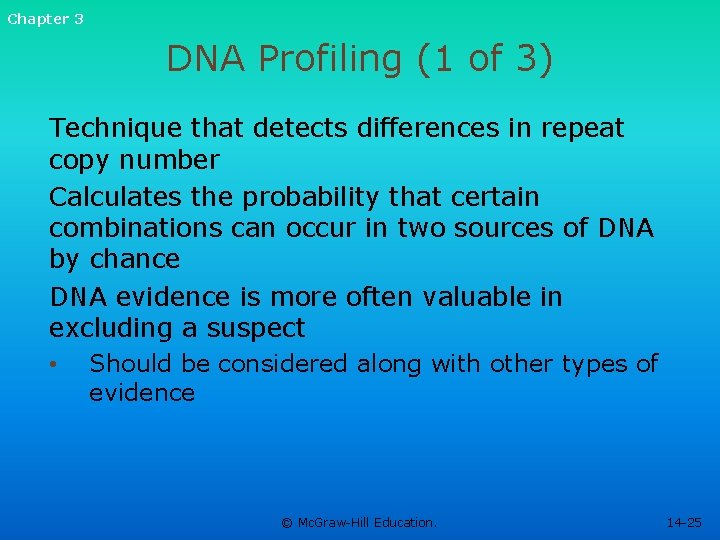
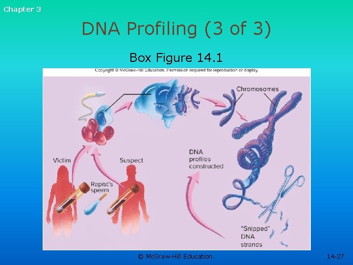
Chapter 3 DNA Profiling (1 of 3) Technique that detects differences in repeat copy number Calculates the probability that certain combinations can occur in two sources of DNA by chance DNA evidence is more often valuable in excluding a suspect • Should be considered along with other types of evidence © Mc. Graw-Hill Education. 14 -25

Chapter 3 DNA Profiling (2 of 3) Developed in the 1980 s by British geneticist Sir Alec Jeffreys Also called DNA fingerprinting Identifies individuals Used in forensics, agriculture, paternity testing, and historical investigations © Mc. Graw-Hill Education. 14 -26

Chapter 3 DNA Profiling (3 of 3) Box Figure 14. 1 © Mc. Graw-Hill Education. 14 -27

Chapter 3 Comparing DNA Repeats Figure 14. 7 © Mc. Graw-Hill Education. 14 -28

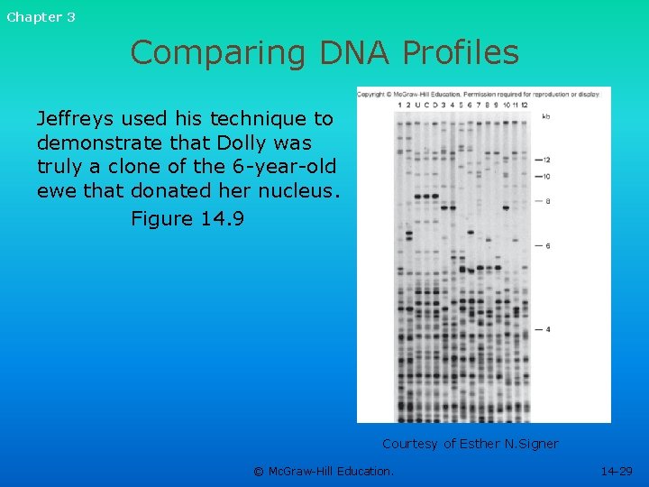
Chapter 3 Comparing DNA Profiles Jeffreys used his technique to demonstrate that Dolly was truly a clone of the 6 -year-old ewe that donated her nucleus. Figure 14. 9 Courtesy of Esther N. Signer © Mc. Graw-Hill Education. 14 -29

Chapter 3 DNA Profiling Technique Blood sample is collected from suspect. White blood cells release DNA. Restriction enzymes cut DNA. Electrophoresis aligns fragments by size. Pattern of DNA fragments transferred to a nylon sheet. Exposed to radioactive probes Probes bind to DNA Sheet placed against X-ray film Pattern of bands constitutes DNA profile Identify individuals © Mc. Graw-Hill Education. 14 -30

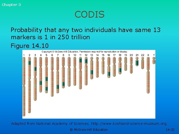
Chapter 3 DNA Sources DNA can be obtained from any cell with a nucleus. STRs are used when DNA is scarce. If DNA is extremely damaged, mitochondrial DNA (mt. DNA) is often used. For forensics, the FBI developed the Combined DNA Index System (CODIS). • Uses 13 STRs © Mc. Graw-Hill Education. 14 -31

Chapter 3 CODIS Probability that any two individuals have same 13 markers is 1 in 250 trillion Figure 14. 10 Adapted from National Academy of Sciences. http: //www. koshland-science-museum. org. © Mc. Graw-Hill Education. 14 -32

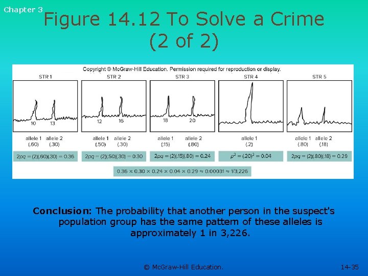
Chapter 3 Population Statistics Used to Interpret DNA Profiles Power of DNA profiling is greatly expanded by tracking repeats in different chromosomes. Number of copies of a repeat are assigned probabilities based on their observed frequency in a population. Product rule is then used to calculate probability of a certain repeat combination. © Mc. Graw-Hill Education. 14 -33

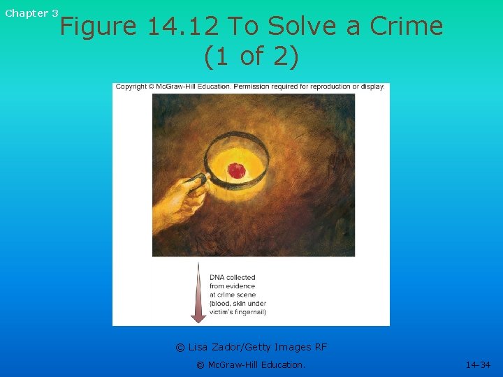
Chapter 3 Figure 14. 12 To Solve a Crime (1 of 2) © Lisa Zador/Getty Images RF © Mc. Graw-Hill Education. 14 -34

Chapter 3 Figure 14. 12 To Solve a Crime (2 of 2) Conclusion: The probability that another person in the suspect's population group has the same pattern of these alleles is approximately 1 in 3, 226. © Mc. Graw-Hill Education. 14 -35

Chapter 3 Using DNA Profiling to Identify Victims Recent examples of large-scale disasters: • • • World Trade Center attack (2001) Indian Ocean Tsunami (2004) Hurricane Katrina (2005) © Mc. Graw-Hill Education. 14 -36

Chapter 3 Challenges to DNA Profiling Table 14. 5 Challenges to DNA Profiling in Mass Disasters Climate that hastens decay Inability to reach remains No laboratory facilities Number of casualties Lack of relatives Destruction of personal item evidence Poor DNA quality (too fragmented, scarce, degraded) Lack of availability of DNA probes and statistics for a population © Mc. Graw-Hill Education. 14 -37

Chapter 3 Genetic Privacy Today’s population genetics presents a powerful way to identify individuals Our genomes can vary in more ways than there are people in the world DNA profiling introduces privacy issues • Example: DNA dragnets © Mc. Graw-Hill Education. 14 -38

End of Presentation © Mc. Graw-Hill Education. All rights reserved. Authorized only for instructor use in the classroom. No reproduction or further distribution permitted without the prior written consent of Mc. Graw-Hill Education. 14 -39