Hierarchical Clustering Produces a set of nested clusters

Hierarchical Clustering • Produces a set of nested clusters organized as a hierarchical tree • Can be visualized as a dendrogram – A tree like diagram that records the sequences of merges or splits

Strengths of Hierarchical Clustering • Do not have to assume any particular number of clusters – Any desired number of clusters can be obtained by ‘cutting’ the dendogram at the proper level • They may correspond to meaningful taxonomies – Example in biological sciences (e. g. , animal kingdom, phylogeny reconstruction, …)

Hierarchical Clustering • Two main types of hierarchical clustering – Agglomerative: • Start with the points as individual clusters • At each step, merge the closest pair of clusters until only one cluster (or k clusters) left – Divisive: • Start with one, all-inclusive cluster • At each step, split a cluster until each cluster contains a point (or there are k clusters) • Traditional hierarchical algorithms use a similarity or distance matrix – Merge or split one cluster at a time

Agglomerative Clustering Algorithm • More popular hierarchical clustering technique • Basic algorithm is straightforward 1. 2. 3. 4. 5. 6. • Compute the proximity matrix Let each data point be a cluster Repeat Merge the two closest clusters Update the proximity matrix Until only a single cluster remains Key operation is the computation of the proximity of two clusters – Different approaches to defining the distance between clusters distinguish the different algorithms

Single Link or Min Proximity Matrix: Minimum of the distance (Maximum of the similarity) between any two points in the two different clusters

The distance between points 3 and 6 is 0. 11

Complete Link or Max Proximity Matrix: Maximum of the distance (Minimum of the similarity) between any two points in the two different clusters

because

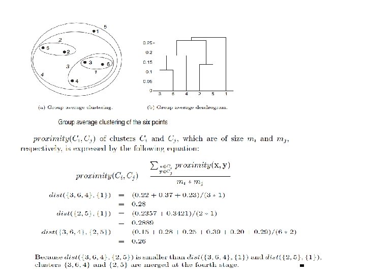
Group Average Proximity Matrix: average pairwise proximity among all pairs of points in the different clusters Intermediate approach between the single and complete link approaches

Ward’s Method Proximity Matrix: the squared error that results when two clusters are merged