Extremely Competitive Markets Part 1 Closed Economies Characteristics

Extremely Competitive Markets Part 1: Closed Economies

Characteristics of Extremely Competitive Markets Many buyers and sellers, or “Easy” entry and exit in the presence of significant extranormal profits Little or no product differentiation Price takers

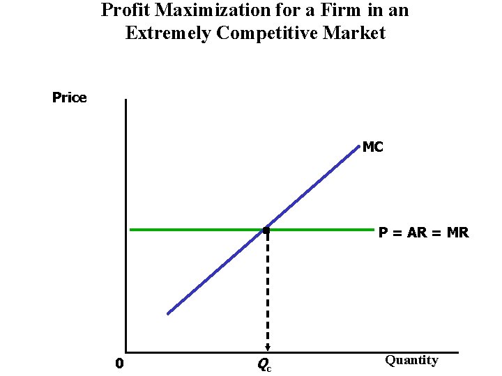
Profit Maximization for a Firm in an Extremely Competitive Market Price MC P = AR = MR 0 Qc Quantity

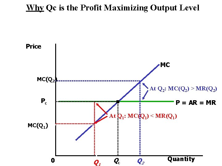
Why Qc is the Profit Maximizing Output Level Price MC MC(Q 2) At Q 2: MC(Q 2) > MR(Q 2) Pc P = AR = MR At Q 1: MC(Q 1) < MR(Q 1) MC(Q 1) 0 Q Qc Q 2 Quantity

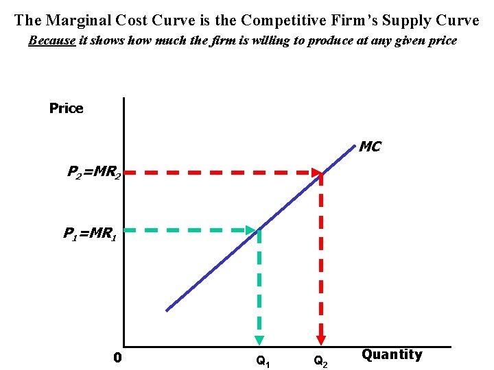
The Marginal Cost Curve is the Competitive Firm’s Supply Curve Because it shows how much the firm is willing to produce at any given price Price MC P 2=MR 2 P 1=MR 1 0 Q 1 Q 2 Quantity

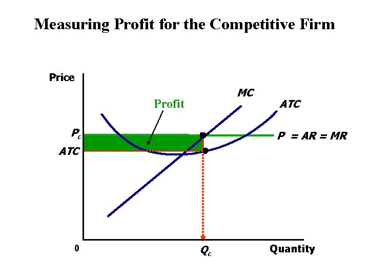
Measuring Profit for the Competitive Firm Price MC Profit Pc ATC P = AR = MR ATC 0 Qc Quantity

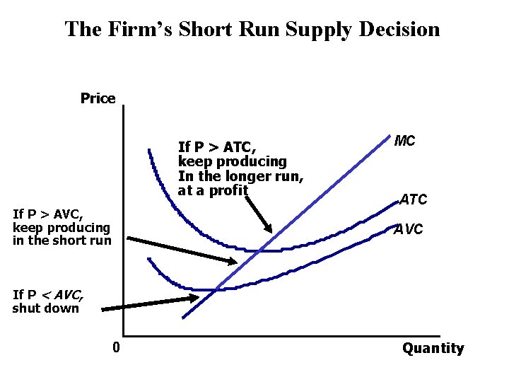
The Firm’s Short Run Supply Decision Price If P > ATC, keep producing In the longer run, at a profit If P > AVC, keep producing in the short run MC ATC AVC If P < AVC, shut down 0 Quantity

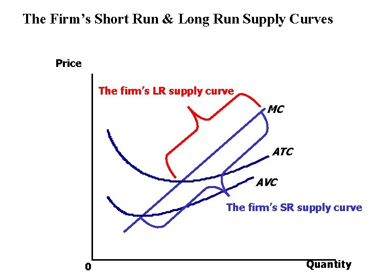
The Firm’s Short Run & Long Run Supply Curves Price The firm’s LR supply curve MC ATC AVC The firm’s SR supply curve 0 Quantity

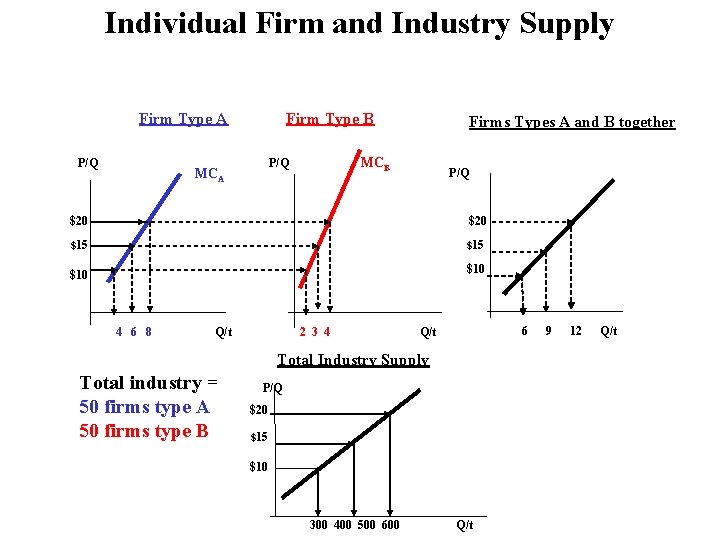
Individual Firm and Industry Supply Firm Type A P/Q Firm Type B MCB P/Q MCA Firms Types A and B together P/Q $20 $15 $10 4 6 8 Q/t 2 3 4 6 Q/t Total Industry Supply Total industry = 50 firms type A 50 firms type B P/Q $20 $15 $10 300 400 500 600 Q/t 9 12 Q/t

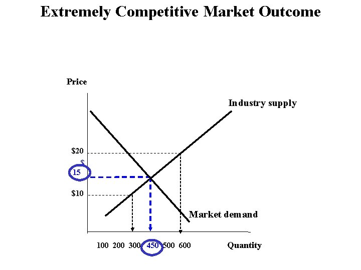
Extremely Competitive Market Outcome Price Industry supply $20 $ 15 $10 Market demand 100 200 300 450 500 600 Quantity

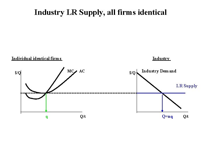
Industry LR Supply, all firms identical Individual identical firms Industry MC $/Q AC $/Q Industry Demand LR Supply q Q/t Q=nq Q/t

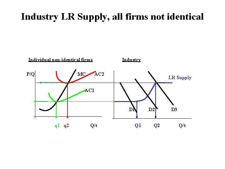
Industry LR Supply, all firms not identical Individual non-identical firms P/Q MC Industry AC 2 LR Supply AC 1 D 1 q 2 Q/t Q 1 D 2 Q 2 D 3 Q/t

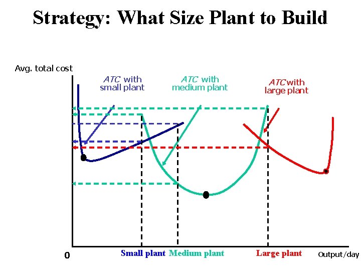
Strategy: What Size Plant to Build Avg. total cost ATC with small plant 0 ATC with medium plant Small plant Medium plant ATC with large plant Large plant Output/day

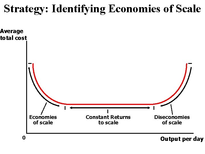
Strategy: Identifying Economies of Scale Average total cost Economies of scale 0 Constant Returns to scale Diseconomies of scale Output per day

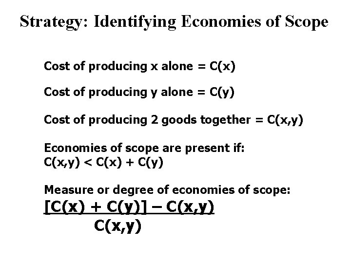
Strategy: Identifying Economies of Scope Cost of producing x alone = C(x) Cost of producing y alone = C(y) Cost of producing 2 goods together = C(x, y) Economies of scope are present if: C(x, y) < C(x) + C(y) Measure or degree of economies of scope: [C(x) + C(y)] – C(x, y)