Evolutionary Computing Chapter 5 Chapter 5 Fitness Selection

Evolutionary Computing Chapter 5

Chapter 5: Fitness, Selection and Population Management • Selection is second fundamental force for evolutionary systems • Components exist of: - Population management models - Selection operators - Preserving diversity 2 / 32

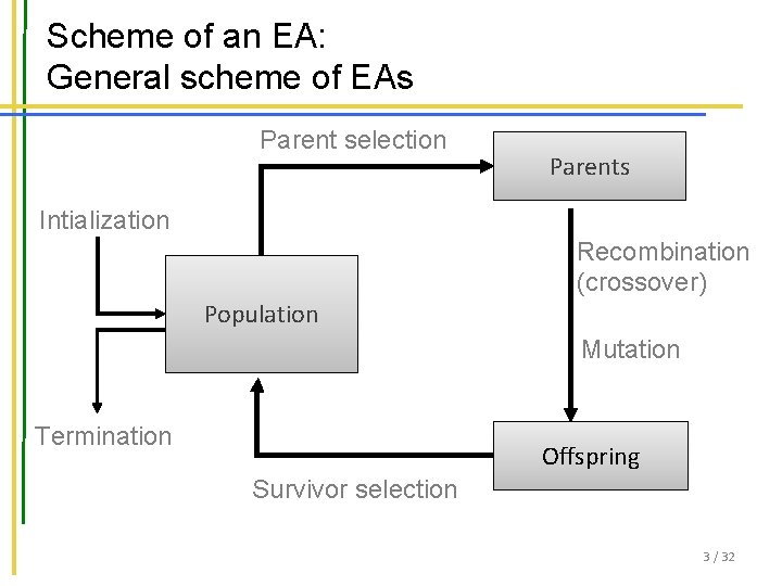
Scheme of an EA: General scheme of EAs Parent selection Parents Intialization Recombination (crossover) Population Mutation Termination Offspring Survivor selection 3 / 32

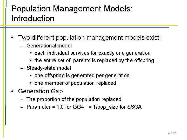
Population Management Models: Introduction • Two different population management models exist: – Generational model • each individual survives for exactly one generation • the entire set of parents is replaced by the offspring – Steady-state model • one offspring is generated per generation • one member of population replaced • Generation Gap – The proportion of the population replaced – Parameter = 1. 0 for GGA, = 1/pop_size for SSGA 4 / 32

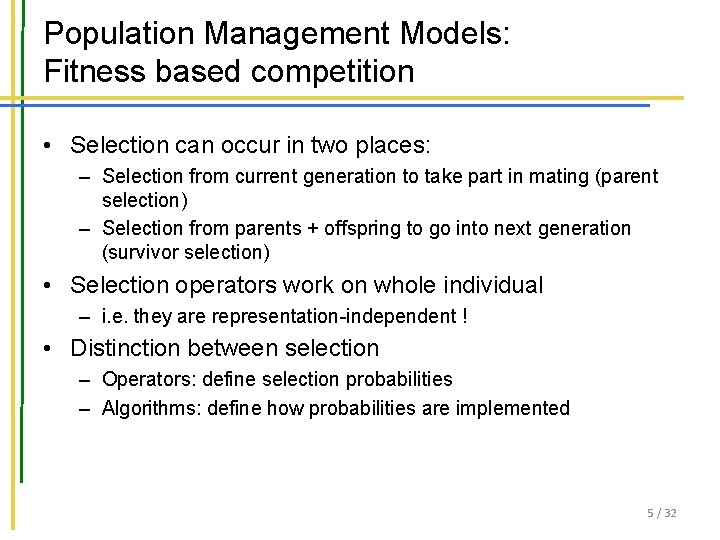
Population Management Models: Fitness based competition • Selection can occur in two places: – Selection from current generation to take part in mating (parent selection) – Selection from parents + offspring to go into next generation (survivor selection) • Selection operators work on whole individual – i. e. they are representation-independent ! • Distinction between selection – Operators: define selection probabilities – Algorithms: define how probabilities are implemented 5 / 32

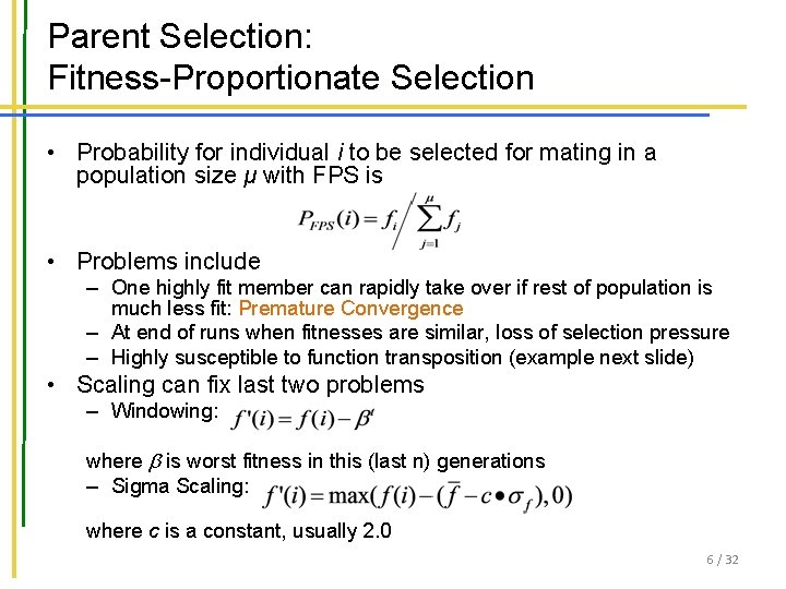
Parent Selection: Fitness-Proportionate Selection • Probability for individual i to be selected for mating in a population size μ with FPS is • Problems include – One highly fit member can rapidly take over if rest of population is much less fit: Premature Convergence – At end of runs when fitnesses are similar, loss of selection pressure – Highly susceptible to function transposition (example next slide) • Scaling can fix last two problems – Windowing: where is worst fitness in this (last n) generations – Sigma Scaling: where c is a constant, usually 2. 0 6 / 32

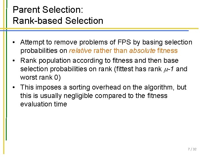
Parent Selection: Rank-based Selection • Attempt to remove problems of FPS by basing selection probabilities on relative rather than absolute fitness • Rank population according to fitness and then base selection probabilities on rank (fittest has rank -1 and worst rank 0) • This imposes a sorting overhead on the algorithm, but this is usually negligible compared to the fitness evaluation time 7 / 32

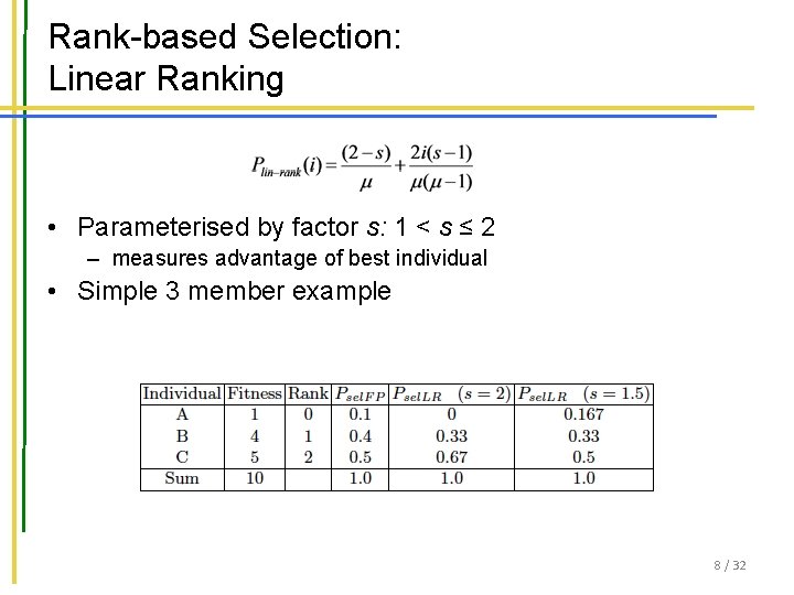
Rank-based Selection: Linear Ranking • Parameterised by factor s: 1 < s ≤ 2 – measures advantage of best individual • Simple 3 member example 8 / 32

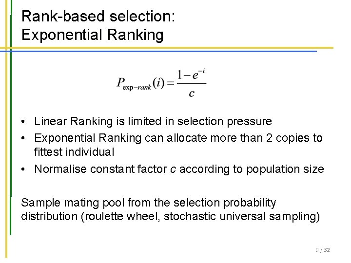
Rank-based selection: Exponential Ranking • Linear Ranking is limited in selection pressure • Exponential Ranking can allocate more than 2 copies to fittest individual • Normalise constant factor c according to population size Sample mating pool from the selection probability distribution (roulette wheel, stochastic universal sampling) 9 / 32

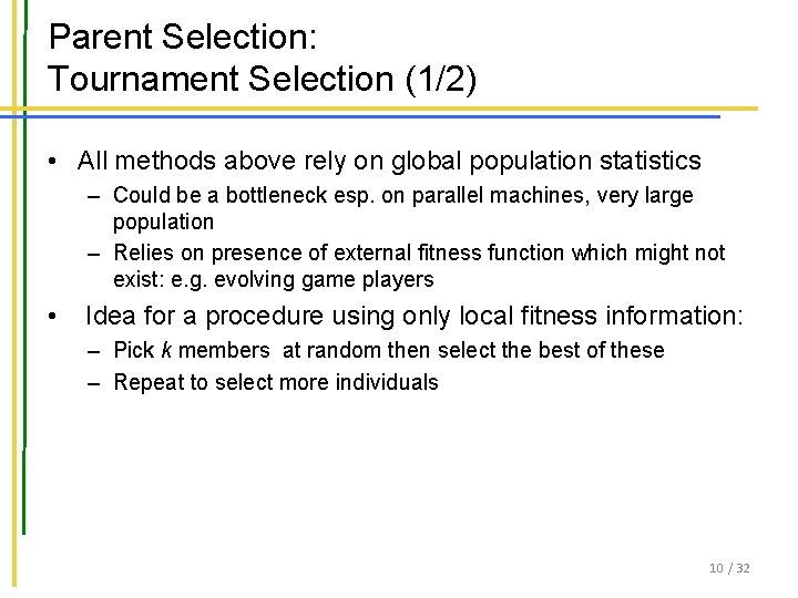
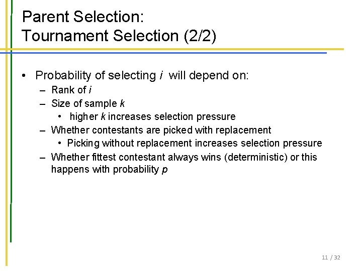
Parent Selection: Tournament Selection (1/2) • All methods above rely on global population statistics – Could be a bottleneck esp. on parallel machines, very large population – Relies on presence of external fitness function which might not exist: e. g. evolving game players • Idea for a procedure using only local fitness information: – Pick k members at random then select the best of these – Repeat to select more individuals 10 / 32

Parent Selection: Tournament Selection (2/2) • Probability of selecting i will depend on: – Rank of i – Size of sample k • higher k increases selection pressure – Whether contestants are picked with replacement • Picking without replacement increases selection pressure – Whether fittest contestant always wins (deterministic) or this happens with probability p 11 / 32

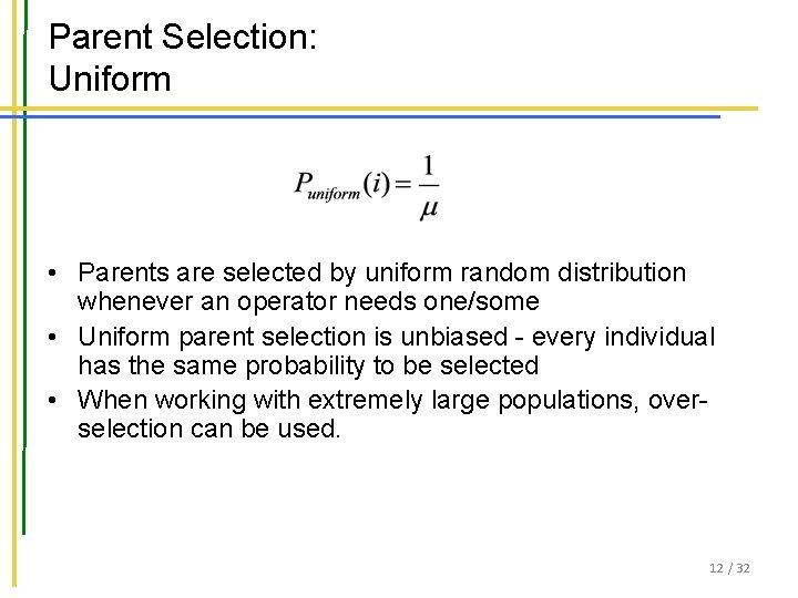
Parent Selection: Uniform • Parents are selected by uniform random distribution whenever an operator needs one/some • Uniform parent selection is unbiased - every individual has the same probability to be selected • When working with extremely large populations, overselection can be used. 12 / 32

Survivor Selection • Managing the process of reducing the working memory of the EA from a set of μ parents and λ offspring to a set of μ individuals forming the next generation • The parent selection mechanisms can also be used for selecting survivors • Survivor selection can be divided into two approaches: – Age-Based Selection • Fitness is not taken into account • In SSGA can implement as “delete-random” (not recommended) or as first-in-first-out (a. k. a. delete-oldest) – Fitness-Based Replacement 13 / 32

Fitness-based replacement (1/2) • Elitism – Always keep at least one copy of the fittest solution so far – Widely used in both population models (GGA, SSGA) • GENITOR: a. k. a. “delete-worst” – From Whitley’s original Steady-State algorithm (he also used linear ranking for parent selection) – Rapid takeover: use with large populations or “no duplicates” policy • Round-robin tournament – P(t): parents, P’(t): offspring – Pairwise competitions in round-robin format: • Each solution x from P(t) P’(t) is evaluated against q other randomly chosen solutions • For each comparison, a "win" is assigned if x is better than its opponent • The solutions with the greatest number of wins are retained to be parents of the next generation – Parameter q allows tuning selection pressure – Typically q = 10 14 / 32

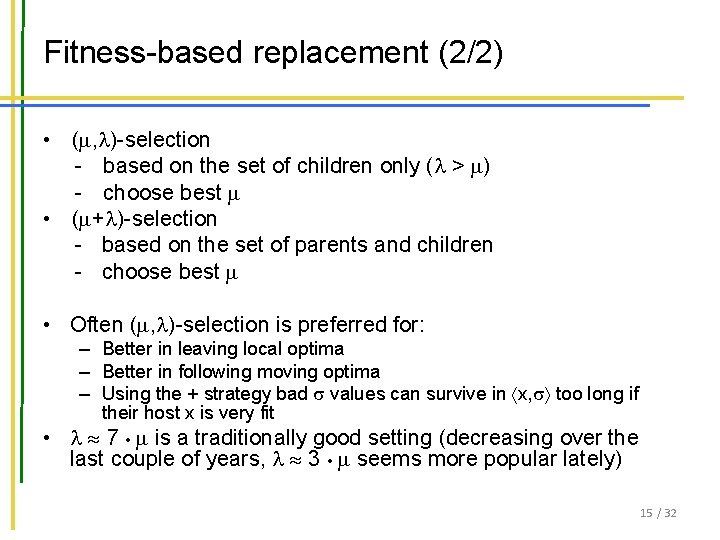
Fitness-based replacement (2/2) • ( , )-selection - based on the set of children only ( > ) - choose best • ( + )-selection - based on the set of parents and children - choose best • Often ( , )-selection is preferred for: – Better in leaving local optima – Better in following moving optima – Using the + strategy bad values can survive in x, too long if their host x is very fit • 7 • is a traditionally good setting (decreasing over the last couple of years, 3 • seems more popular lately) 15 / 32

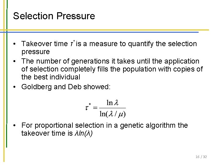
Selection Pressure • Takeover time τ* is a measure to quantify the selection pressure • The number of generations it takes until the application of selection completely fills the population with copies of the best individual • Goldberg and Deb showed: • For proportional selection in a genetic algorithm the takeover time is λln(λ) 16 / 32

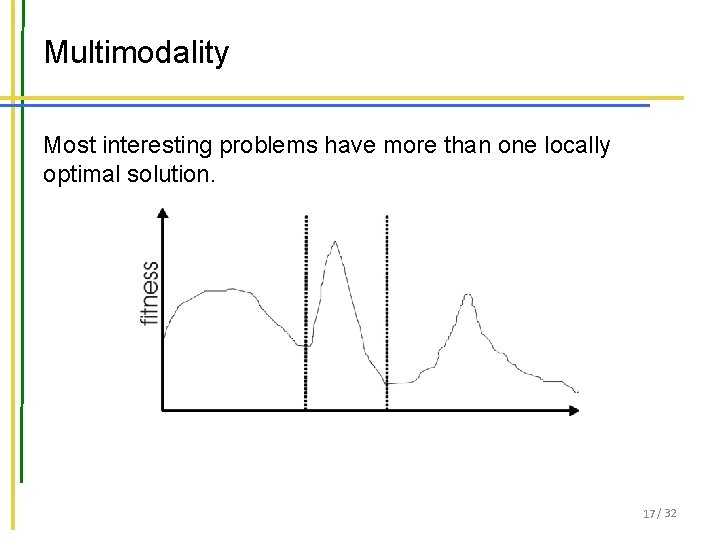
Multimodality Most interesting problems have more than one locally optimal solution. 17 / 32

Multimodality: Genetic Drift • Finite population with global mixing and selection eventually convergence around one optimum • Why? • Often might want to identify several possible peaks • Sub-optimum can be more attractive 18 / 32

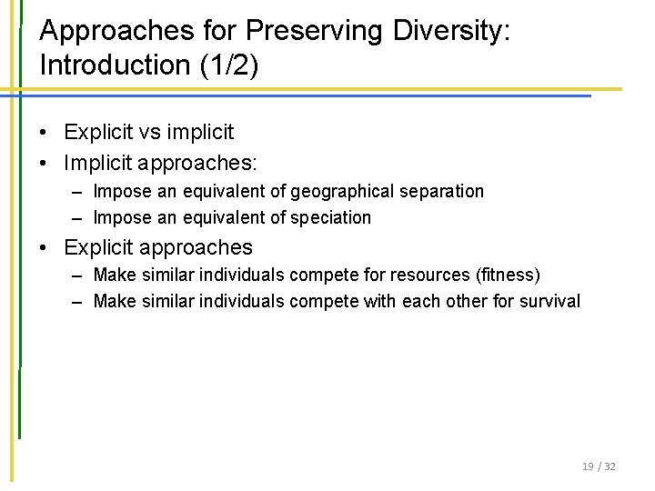
Approaches for Preserving Diversity: Introduction (1/2) • Explicit vs implicit • Implicit approaches: – Impose an equivalent of geographical separation – Impose an equivalent of speciation • Explicit approaches – Make similar individuals compete for resources (fitness) – Make similar individuals compete with each other for survival 19 / 32

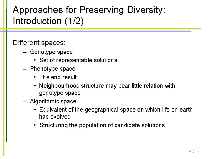
Approaches for Preserving Diversity: Introduction (1/2) Different spaces: – Genotype space • Set of representable solutions – Phenotype space • The end result • Neighbourhood structure may bear little relation with genotype space – Algorithmic space • Equivalent of the geographical space on which life on earth has evolved • Structuring the population of candidate solutions 20 / 32

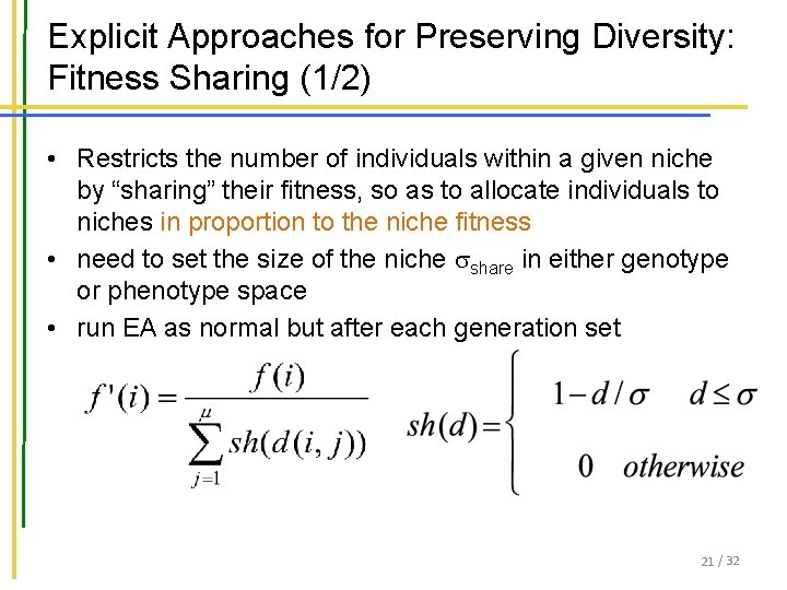
Explicit Approaches for Preserving Diversity: Fitness Sharing (1/2) • Restricts the number of individuals within a given niche by “sharing” their fitness, so as to allocate individuals to niches in proportion to the niche fitness • need to set the size of the niche share in either genotype or phenotype space • run EA as normal but after each generation set 21 / 32

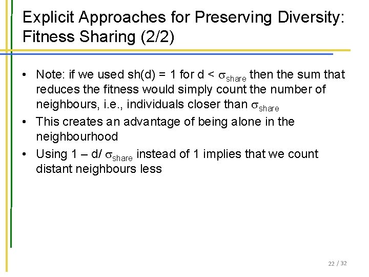
Explicit Approaches for Preserving Diversity: Fitness Sharing (2/2) • Note: if we used sh(d) = 1 for d < share then the sum that reduces the fitness would simply count the number of neighbours, i. e. , individuals closer than share • This creates an advantage of being alone in the neighbourhood • Using 1 – d/ share instead of 1 implies that we count distant neighbours less 22 / 32

Explicit Approaches for Preserving Diversity: Crowding (1/2) • Attempts to distribute individuals evenly amongst niches • relies on the assumption that offspring will tend to be close to parents • uses a distance metric in ph/genotype space • randomly shuffle and pair parents, produce 2 offspring • set up the parent vs. child tournaments such that the intertournament distances are minimal 23 / 32

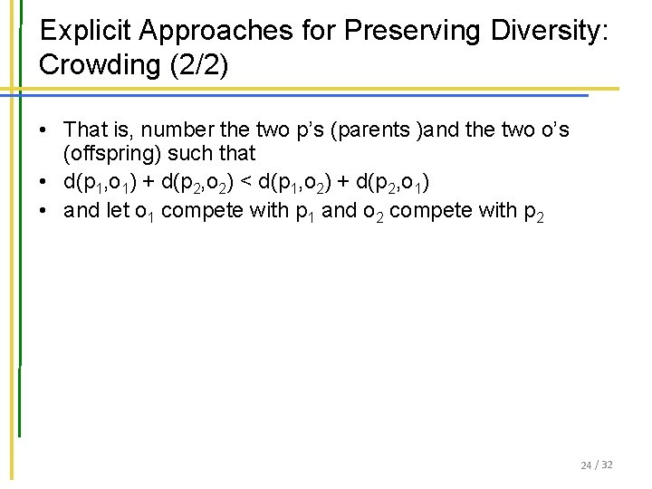
Explicit Approaches for Preserving Diversity: Crowding (2/2) • That is, number the two p’s (parents )and the two o’s (offspring) such that • d(p 1, o 1) + d(p 2, o 2) < d(p 1, o 2) + d(p 2, o 1) • and let o 1 compete with p 1 and o 2 compete with p 2 24 / 32

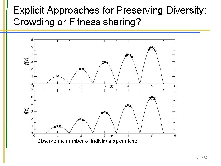
Explicit Approaches for Preserving Diversity: Crowding or Fitness sharing? Observe the number of individuals per niche 25 / 32

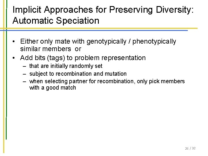
Implicit Approaches for Preserving Diversity: Automatic Speciation • Either only mate with genotypically / phenotypically similar members or • Add bits (tags) to problem representation – that are initially randomly set – subject to recombination and mutation – when selecting partner for recombination, only pick members with a good match 26 / 32

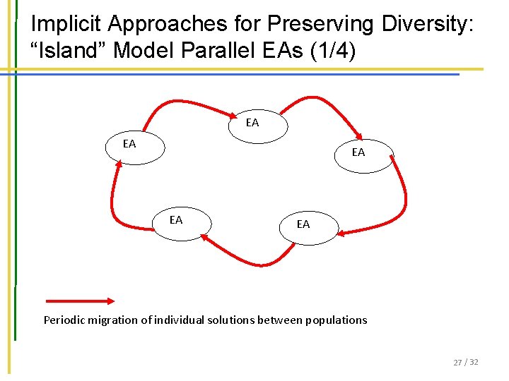
Implicit Approaches for Preserving Diversity: “Island” Model Parallel EAs (1/4) EA EA EA Periodic migration of individual solutions between populations 27 / 32

Implicit Approaches for Preserving Diversity: “Island” Model Parallel EAs (2/4) • Run multiple populations in parallel • After a (usually fixed) number of generations (an Epoch), exchange individuals with neighbours • Repeat until ending criteria met • Partially inspired by parallel/clustered systems 28 / 32

Island Model: Parameters • How often to exchange individuals ? – – too quick and all sub-populations converge to same solution too slow and waste time most authors use range~ 25 -150 generations can do it adaptively (stop each pop when no improvement for (say) 25 generations) • How many, which individuals to exchange ? – usually ~2 -5, but depends on population size. – Copied vs moved – Martin et al found that better to exchange randomly selected individuals than best • Operators can differ between the sub-populations 29 / 32

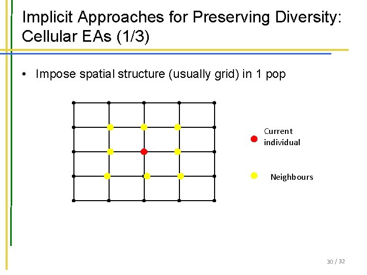
Implicit Approaches for Preserving Diversity: Cellular EAs (1/3) • Impose spatial structure (usually grid) in 1 pop Current individual Neighbours 30 / 32

Implicit Approaches for Preserving Diversity: Cellular EAs (2/3) • Consider each individual to exist on a point on a (usually rectangular toroid) grid • Selection (hence recombination) and replacement happen using concept of a neighbourhood a. k. a. deme • Leads to different parts of grid searching different parts of space, good solutions diffuse across grid over a number of gens 31 / 32

Implicit Approaches for Preserving Diversity: Cellular EAs (3/3) • Assume rectangular grid so each individual has 8 immediate neighbours • Equivalent of 1 generation is: – – – pick individual in pop at random pick one of its neighbours using roulette wheel crossover to produce 1 child, mutate replace individual if fitter circle through population until done 32 / 32