ENGR 2213 Thermodynamics F C Lai School of

ENGR 2213 Thermodynamics F. C. Lai School of Aerospace and Mechanical Engineering University of Oklahoma

Gas Power Cycles Otto Cycle - Ideal cycle for spark-ignition engines Diesel Cycle - Ideal cycle for compression-ignition engines Brayton Cycle - Ideal cycle for gas-turbine engines

Gas Power Cycles Cold Air-Standard Assumptions 1. The working fluid is air which continuously circulates in a closed loop and always behaves as an ideal gas. 2. All the processes which make up the cycle are internally reversible. 3. The combustion process is replaced by a heat addition process from an external source. 4. The exhaust process is replaced by a heat rejection process which restores the air to its initial state. ► Air has constant specific heats which are evaluated at room temperature (25 ºC or 77 ºF).

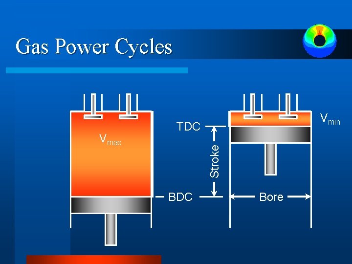
Gas Power Cycles TDC Stroke Vmax Vmin Displacement volume BDC Bore

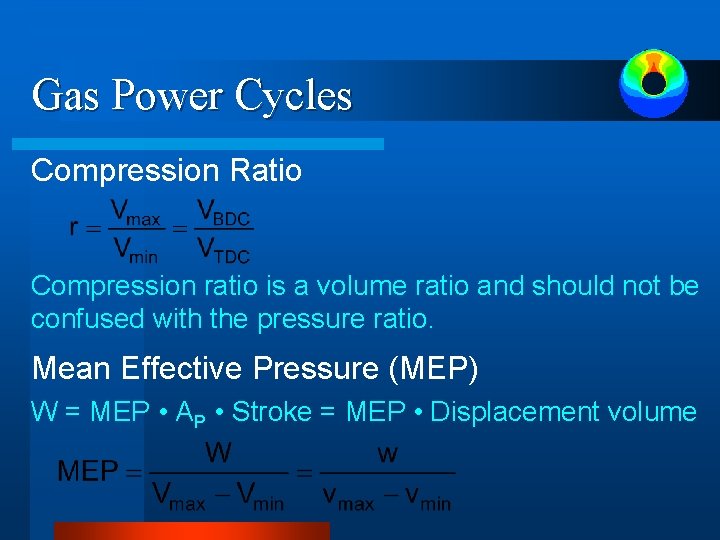
Gas Power Cycles Compression Ratio Compression ratio is a volume ratio and should not be confused with the pressure ratio. Mean Effective Pressure (MEP) W = MEP • AP • Stroke = MEP • Displacement volume

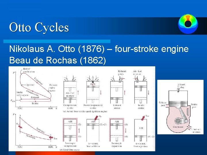
Otto Cycles Nikolaus A. Otto (1876) – four-stroke engine Beau de Rochas (1862)

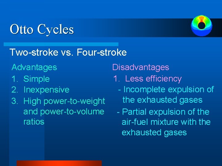
Otto Cycles Two-stroke vs. Four-stroke Advantages Disadvantages 1. Less efficiency 1. Simple - Incomplete expulsion of 2. Inexpensive the exhausted gases 3. High power-to-weight and power-to-volume - Partial expulsion of the ratios air-fuel mixture with the exhausted gases

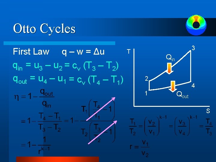
Otto Cycles First Law q – w = Δu qin = u 3 – u 2 = cv (T 3 – T 2) qout = u 4 – u 1 = cv (T 4 – T 1) 3 T Qin 2 4 1 Qout S

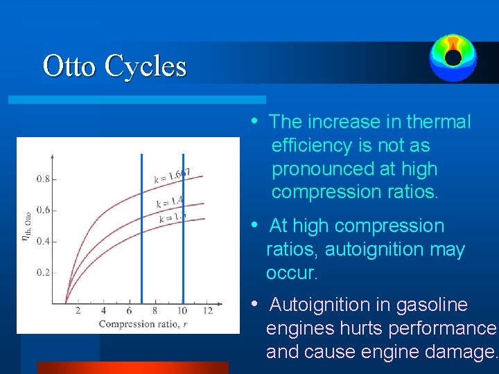
Otto Cycles • The increase in thermal efficiency is not as pronounced at high compression ratios. • At high compression ratios, autoignition may occur. • Autoignition in gasoline engines hurts performance and cause engine damage.

Example 1 An ideal Otto cycle has a compression ratio of 8. At the beginning of the compression process, air is at 100 k. Pa and 17 ºC, and 800 k. J/kg of heat is transferred to air during the constant-volume heat addition process. Accounting for the variation of specific heats of air with temperature, determine (a) the maximum temperature and pressure which occur during the cycle, (b) the net work output, (c) thermal efficiency of this cycle, and (d) the mean effective pressure for the cycle.

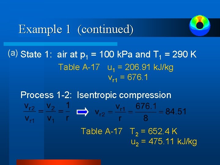
Example 1 (continued) (a) State 1: air at p 1 = 100 k. Pa and T 1 = 290 K Table A-17 u 1 = 206. 91 k. J/kg vr 1 = 676. 1 Process 1 -2: Isentropic compression Table A-17 T 2 = 652. 4 K u 2 = 475. 11 k. J/kg

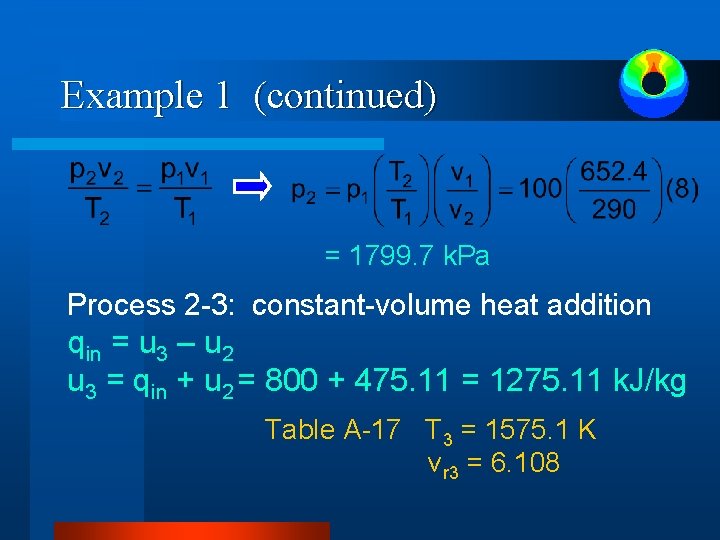
Example 1 (continued) = 1799. 7 k. Pa Process 2 -3: constant-volume heat addition qin = u 3 – u 2 u 3 = qin + u 2 = 800 + 475. 11 = 1275. 11 k. J/kg Table A-17 T 3 = 1575. 1 K vr 3 = 6. 108

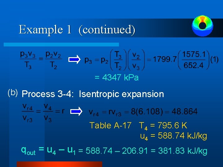
Example 1 (continued) = 4347 k. Pa (b) Process 3 -4: Isentropic expansion Table A-17 T 4 = 795. 6 K u 4 = 588. 74 k. J/kg qout = u 4 – u 1 = 588. 74 – 206. 91 = 381. 83 k. J/kg

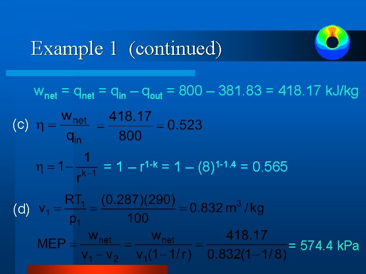
Example 1 (continued) wnet = qin – qout = 800 – 381. 83 = 418. 17 k. J/kg (c) = 1 – r 1 -k = 1 – (8)1 -1. 4 = 0. 565 (d) = 574. 4 k. Pa

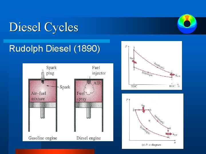
Diesel Cycles Rudolph Diesel (1890)

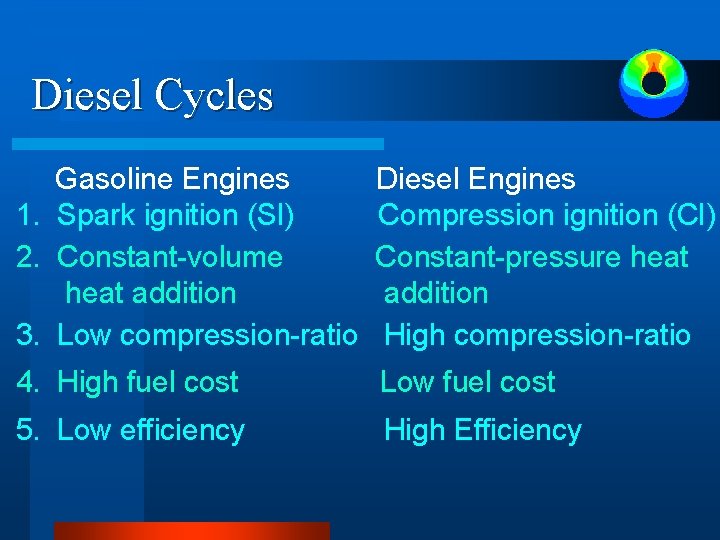
Diesel Cycles Gasoline Engines 1. Spark ignition (SI) 2. Constant-volume heat addition 3. Low compression-ratio Diesel Engines Compression ignition (CI) Constant-pressure heat addition High compression-ratio 4. High fuel cost Low fuel cost 5. Low efficiency High Efficiency

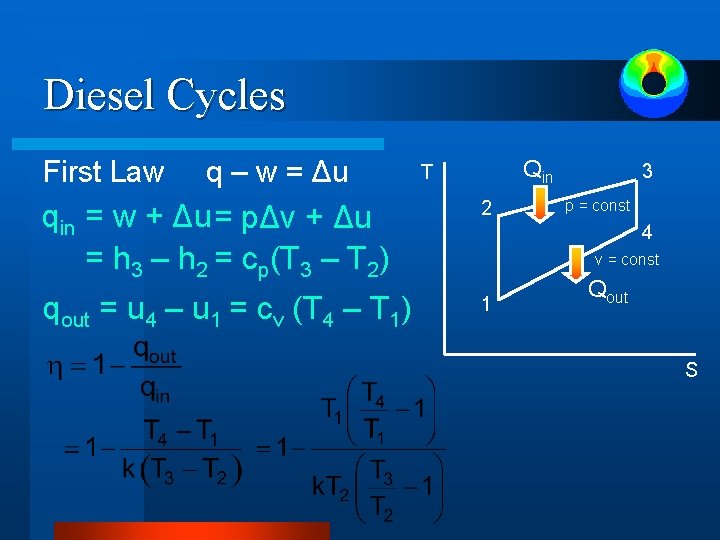
Diesel Cycles First Law q – w = Δu Qin T qin = w + Δu = pΔv + Δu = h 3 – h 2 = cp(T 3 – T 2) 2 qout = u 4 – u 1 = cv (T 4 – T 1) 1 3 p = const 4 v = const Qout S

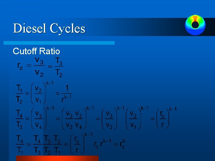
Diesel Cycles Cutoff Ratio

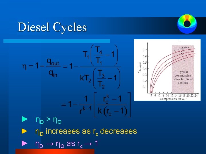
Diesel Cycles ► ηD > ηO ► ηD increases as rc decreases ► ηD → ηO as rc → 1

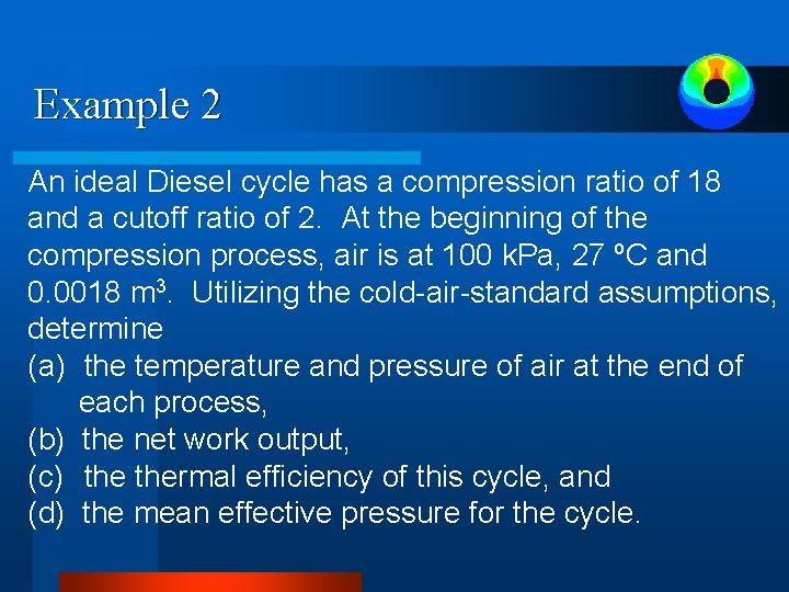
Example 2 An ideal Diesel cycle has a compression ratio of 18 and a cutoff ratio of 2. At the beginning of the compression process, air is at 100 k. Pa, 27 ºC and 0. 0018 m 3. Utilizing the cold-air-standard assumptions, determine (a) the temperature and pressure of air at the end of each process, (b) the net work output, (c) thermal efficiency of this cycle, and (d) the mean effective pressure for the cycle.

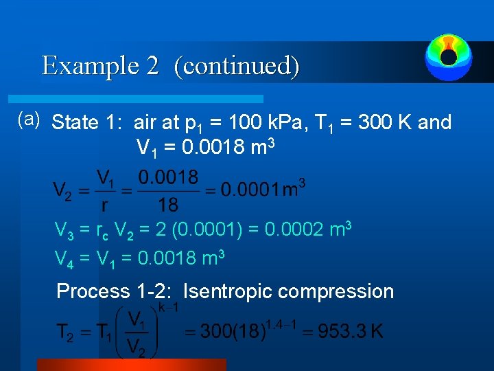
Example 2 (continued) (a) State 1: air at p 1 = 100 k. Pa, T 1 = 300 K and V 1 = 0. 0018 m 3 V 3 = rc V 2 = 2 (0. 0001) = 0. 0002 m 3 V 4 = V 1 = 0. 0018 m 3 Process 1 -2: Isentropic compression

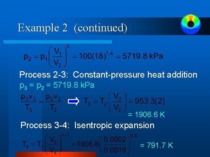
Example 2 (continued) Process 2 -3: Constant-pressure heat addition p 3 = p 2 = 5719. 8 k. Pa = 1906. 6 K Process 3 -4: Isentropic expansion = 791. 7 K

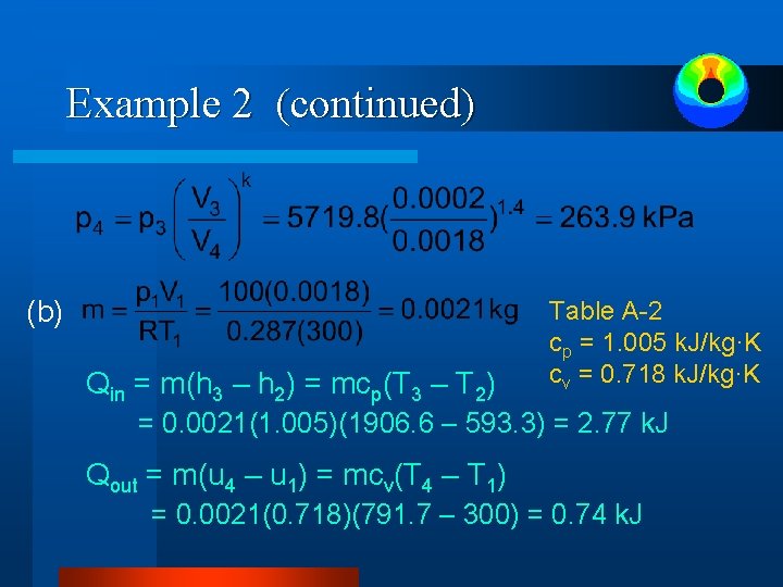
Example 2 (continued) (b) Qin = m(h 3 – h 2) = mcp(T 3 – T 2) Table A-2 cp = 1. 005 k. J/kg·K cv = 0. 718 k. J/kg·K = 0. 0021(1. 005)(1906. 6 – 593. 3) = 2. 77 k. J Qout = m(u 4 – u 1) = mcv(T 4 – T 1) = 0. 0021(0. 718)(791. 7 – 300) = 0. 74 k. J

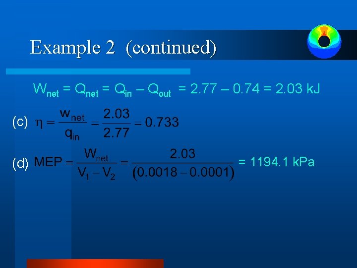
Example 2 (continued) Wnet = Qin – Qout = 2. 77 – 0. 74 = 2. 03 k. J (c) (d) = 1194. 1 k. Pa