ECON 511 International Finance Open Macroeconomy CHAPTER THREE

ECON 511 International Finance & Open Macroeconomy CHAPTER THREE The Monetary Approach to Flexible Exchange Rates

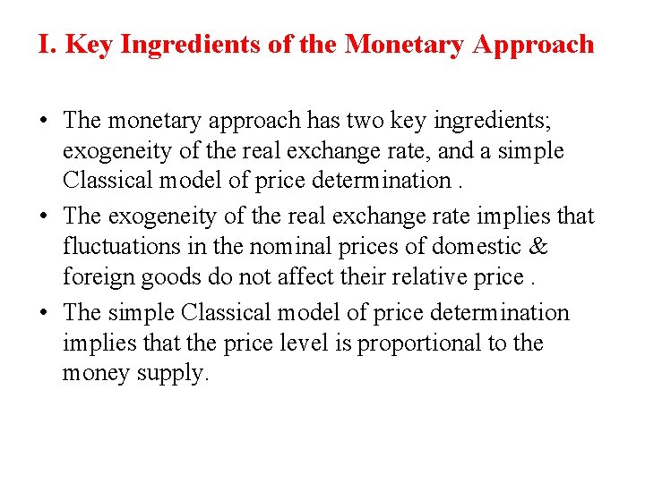
I. Key Ingredients of the Monetary Approach • The monetary approach has two key ingredients; exogeneity of the real exchange rate, and a simple Classical model of price determination. • The exogeneity of the real exchange rate implies that fluctuations in the nominal prices of domestic & foreign goods do not affect their relative price. • The simple Classical model of price determination implies that the price level is proportional to the money supply.

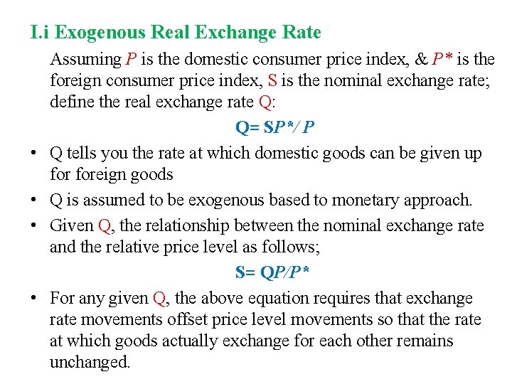
I. i Exogenous Real Exchange Rate • • Assuming P is the domestic consumer price index, & P* is the foreign consumer price index, S is the nominal exchange rate; define the real exchange rate Q: Q= SP*/ P Q tells you the rate at which domestic goods can be given up foreign goods Q is assumed to be exogenous based to monetary approach. Given Q, the relationship between the nominal exchange rate and the relative price level as follows; S= QP/P* For any given Q, the above equation requires that exchange rate movements offset price level movements so that the rate at which goods actually exchange for each other remains unchanged.

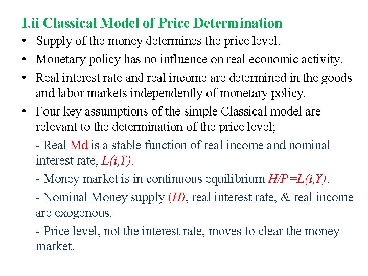
I. ii Classical Model of Price Determination • Supply of the money determines the price level. • Monetary policy has no influence on real economic activity. • Real interest rate and real income are determined in the goods and labor markets independently of monetary policy. • Four key assumptions of the simple Classical model are relevant to the determination of the price level; - Real Md is a stable function of real income and nominal interest rate, L(i, Y). - Money market is in continuous equilibrium H/P=L(i, Y). - Nominal Money supply (H), real interest rate, & real income are exogenous. - Price level, not the interest rate, moves to clear the money market.

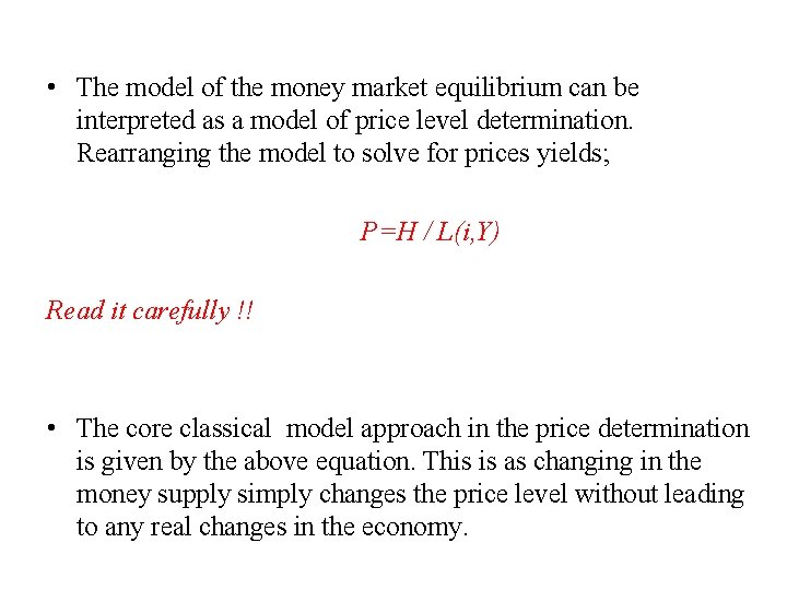
• The model of the money market equilibrium can be interpreted as a model of price level determination. Rearranging the model to solve for prices yields; P=H / L(i, Y) Read it carefully !! • The core classical model approach in the price determination is given by the above equation. This is as changing in the money supply simply changes the price level without leading to any real changes in the economy.

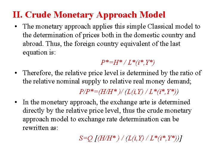
II. Crude Monetary Approach Model • The monetary approach applies this simple Classical model to the determination of prices both in the domestic country and abroad. Thus, the foreign country equivalent of the last equation is: P*=H* / L*(i*, Y*) • Therefore, the relative price level is determined by the ratio of the relative nominal supply to relative real money demand; P/P*=(H/H* )/ (L(i, Y) / L*(i*, Y*)) • In the monetary approach, the exchange arte is determined directly by the relative price level, thus the crude monetary approach model to exchange rate determination can be rewritten as: S=Q [(H/H* ) / (L(i, Y) / L*(i*, Y*))]

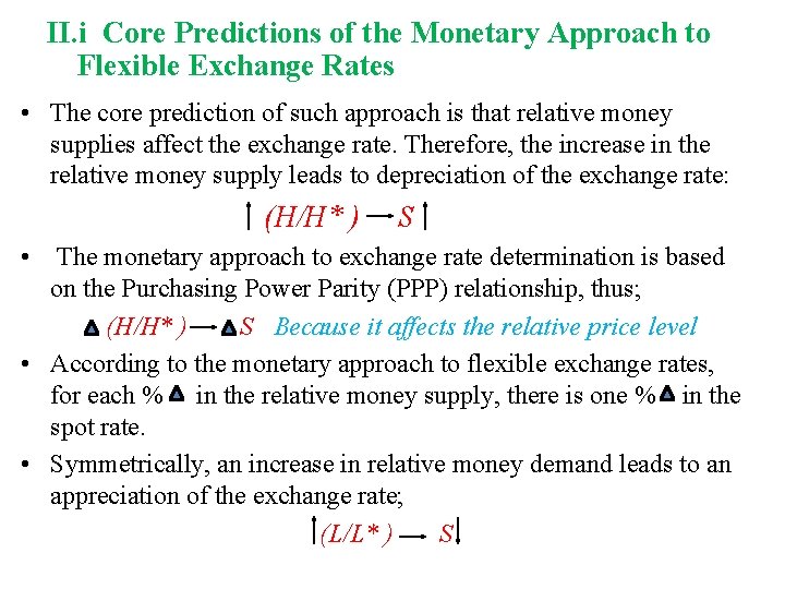
II. i Core Predictions of the Monetary Approach to Flexible Exchange Rates • The core prediction of such approach is that relative money supplies affect the exchange rate. Therefore, the increase in the relative money supply leads to depreciation of the exchange rate: (H/H* ) S • The monetary approach to exchange rate determination is based on the Purchasing Power Parity (PPP) relationship, thus; (H/H* ) S Because it affects the relative price level • According to the monetary approach to flexible exchange rates, for each % in the relative money supply, there is one % in the spot rate. • Symmetrically, an increase in relative money demand leads to an appreciation of the exchange rate; (L/L* ) S

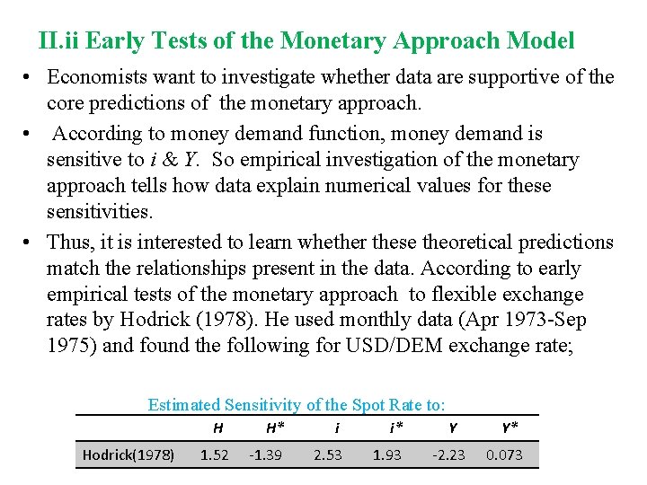
II. ii Early Tests of the Monetary Approach Model • Economists want to investigate whether data are supportive of the core predictions of the monetary approach. • According to money demand function, money demand is sensitive to i & Y. So empirical investigation of the monetary approach tells how data explain numerical values for these sensitivities. • Thus, it is interested to learn whether these theoretical predictions match the relationships present in the data. According to early empirical tests of the monetary approach to flexible exchange rates by Hodrick (1978). He used monthly data (Apr 1973 -Sep 1975) and found the following for USD/DEM exchange rate; Estimated Sensitivity of the Spot Rate to: H Hodrick(1978) 1. 52 H* i i* -1. 39 2. 53 1. 93 Y Y* -2. 23 0. 073

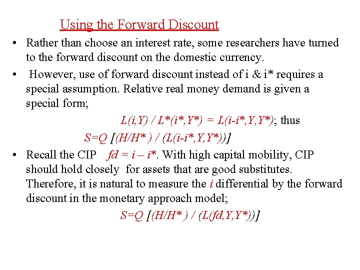
Using the Forward Discount • Rather than choose an interest rate, some researchers have turned to the forward discount on the domestic currency. • However, use of forward discount instead of i & i* requires a special assumption. Relative real money demand is given a special form; L(i, Y) / L*(i*, Y*) = L(i-i*, Y, Y*); thus S=Q [(H/H* ) / (L(i-i*, Y, Y*))] • Recall the CIP fd = i – i*. With high capital mobility, CIP should hold closely for assets that are good substitutes. Therefore, it is natural to measure the i differential by the forward discount in the monetary approach model; S=Q [(H/H* ) / (L(fd, Y, Y*))]

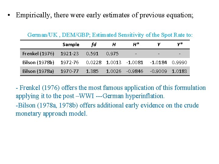
• Empirically, there were early estimates of previous equation; German/UK , DEM/GBP; Estimated Sensitivity of the Spot Rate to: Sample fd H H* Y Y* Frenkel (1976) 1921 -23 0. 591 0. 975 - - - Bilson (1978 b) 1972 -76 0. 0228 1. 0013 -1. 0081 -1. 0184 0. 9990 Bilson (1978 a) 1970 -77 1. 385 -0. 9009 1. 0183 1. 0026 -0. 9846 - Frenkel (1976) offers the most famous application of this formulation applying it to the post –WWI ---German hyperinflation. -Bilson (1978 a, 1978 b) offers additional early evidence on the crude monetary approach model.

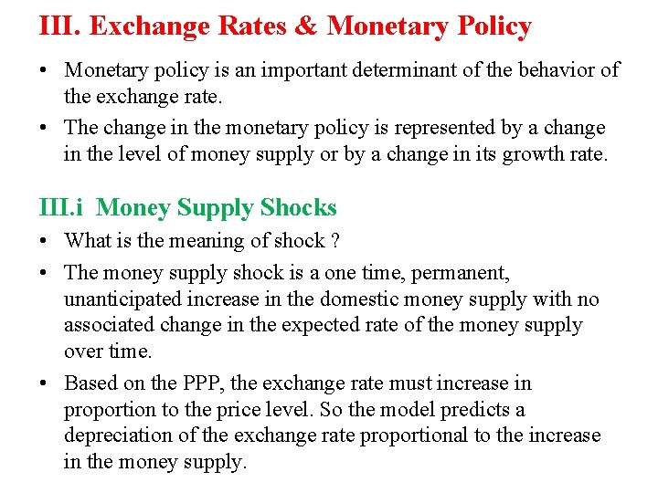
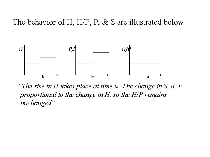
III. Exchange Rates & Monetary Policy • Monetary policy is an important determinant of the behavior of the exchange rate. • The change in the monetary policy is represented by a change in the level of money supply or by a change in its growth rate. III. i Money Supply Shocks • What is the meaning of shock ? • The money supply shock is a one time, permanent, unanticipated increase in the domestic money supply with no associated change in the expected rate of the money supply over time. • Based on the PPP, the exchange rate must increase in proportion to the price level. So the model predicts a depreciation of the exchange rate proportional to the increase in the money supply.

The behavior of H, H/P, P, & S are illustrated below: H P, S t 0 H/P t 0 “The rise in H takes place at time t 0. The change in S, & P proportional to the change in H, so the H/P remains unchanged”

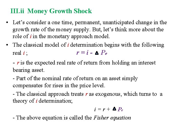
III. ii Money Growth Shock • Let’s consider a one time, permanent, unanticipated change in the growth rate of the money supply. But, let’s think more about the role of i in the monetary approach model. • The classical model of i determination begins with the following real i ; r = i - Pe - r is the expected real rate of return from holding an interest bearing asset. - Part of the nominal rate of return on an asset simply compensates for rises in the price level. - The classical approach treats r as exogenous, which turns to a theory of i determination; i = r + Pe - The above equation is called the Fisher equation

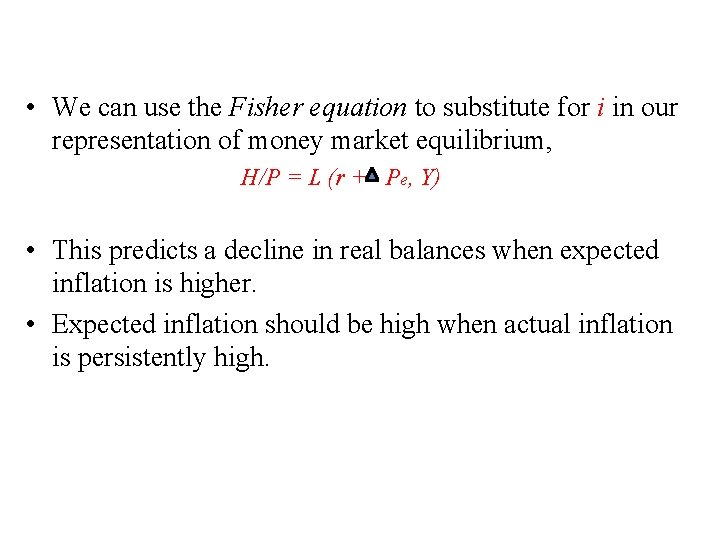
• We can use the Fisher equation to substitute for i in our representation of money market equilibrium, H/P = L (r + Pe, Y) • This predicts a decline in real balances when expected inflation is higher. • Expected inflation should be high when actual inflation is persistently high.

IV. Exchange Rate & Anticipated Monetary Policy • Let’s consider what happens when changes in policy are anticipated. IV. i An Anticipated Change in the Money Supply • Let’s consider a one time, permanent, anticipated increase in the level of the money supply. Note this shock is known in advance.

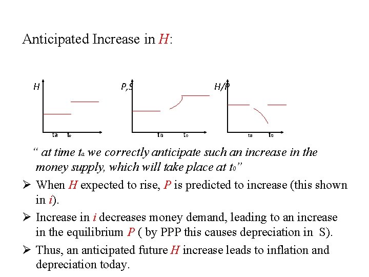
Anticipated Increase in H: H P, S ta t 0 H/P ta t 0 “ at time ta we correctly anticipate such an increase in the money supply, which will take place at t 0” Ø When H expected to rise, P is predicted to increase (this shown in i). Ø Increase in i decreases money demand, leading to an increase in the equilibrium P ( by PPP this causes depreciation in S). Ø Thus, an anticipated future H increase leads to inflation and depreciation today.

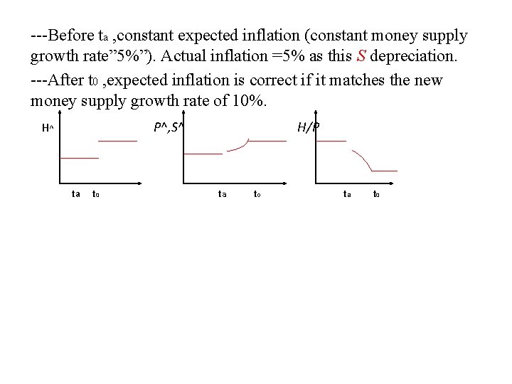
IV. ii An Anticipated Change in the Money Growth • Suppose at time ta , we correctly anticipate a one time, permanent increase in the rate of growth of money supply ( annual growth 0 -10%). • So, the P & inflation rate must respond immediately to our expectations of a future policy change. Also because of PPP, S responds. • Recall, increases in expected inflation immediately increase the S ( by reducing relative money demand & thereby increasing the relative price level).

---Before ta , constant expected inflation (constant money supply growth rate” 5%”). Actual inflation =5% as this S depreciation. ---After t 0 , expected inflation is correct if it matches the new money supply growth rate of 10%. P^, S^ H^ ta t 0 H/P ta t 0