ECE 471 571 Pattern Recognition Lecture 7 Dimensionality

ECE 471 -571 – Pattern Recognition Lecture 7 – Dimensionality Reduction – Principal Component Analysis Hairong Qi, Gonzalez Family Professor Electrical Engineering and Computer Science University of Tennessee, Knoxville http: //www. eecs. utk. edu/faculty/qi Email: hqi@utk. edu

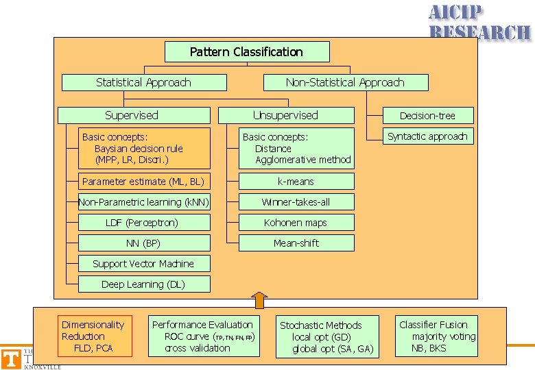
Pattern Classification Statistical Approach Supervised Basic concepts: Baysian decision rule (MPP, LR, Discri. ) Non-Statistical Approach Unsupervised Basic concepts: Distance Agglomerative method Parameter estimate (ML, BL) k-means Non-Parametric learning (k. NN) Winner-takes-all LDF (Perceptron) Kohonen maps NN (BP) Mean-shift Decision-tree Syntactic approach Support Vector Machine Deep Learning (DL) Dimensionality Reduction FLD, PCA Performance Evaluation ROC curve (TP, TN, FP) cross validation Stochastic Methods local opt (GD) global opt (SA, GA) Classifier Fusion majority voting NB, BKS

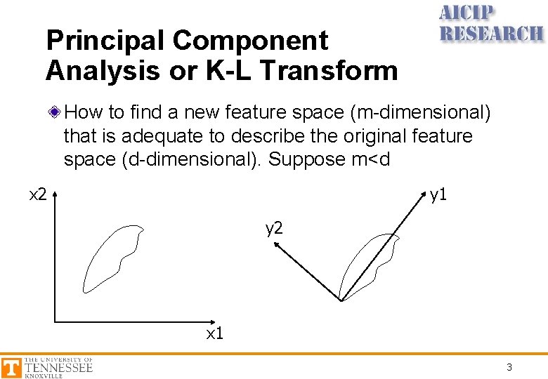
Principal Component Analysis or K-L Transform How to find a new feature space (m-dimensional) that is adequate to describe the original feature space (d-dimensional). Suppose m<d x 2 y 1 y 2 x 1 3

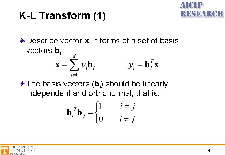
K-L Transform (1) Describe vector x in terms of a set of basis vectors bi. The basis vectors (bi) should be linearly independent and orthonormal, that is, 4

K-L Transform (2) Suppose we wish to ignore all but m (m<d) components of y and still represent x, although with some error. We will thus calculate the first m elements of y and replace the others with constants Error: 5

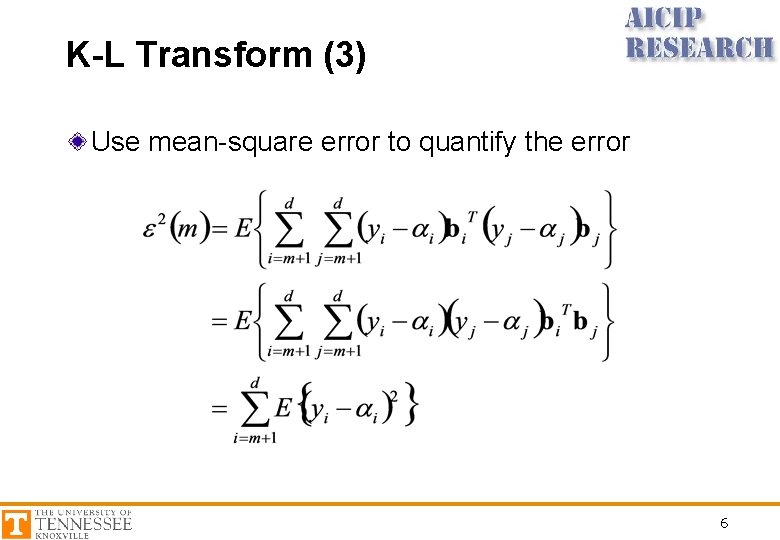
K-L Transform (3) Use mean-square error to quantify the error 6

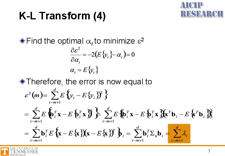
K-L Transform (4) Find the optimal ai to minimize e 2 Therefore, the error is now equal to 7

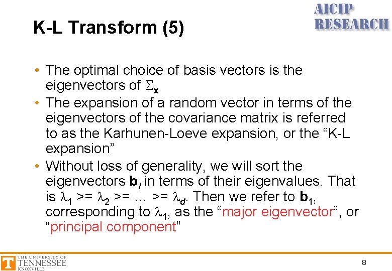
K-L Transform (5) • The optimal choice of basis vectors is the eigenvectors of Sx • The expansion of a random vector in terms of the eigenvectors of the covariance matrix is referred to as the Karhunen-Loeve expansion, or the “K-L expansion” • Without loss of generality, we will sort the eigenvectors bi in terms of their eigenvalues. That is l 1 >= l 2 >= … >= ld. Then we refer to b 1, corresponding to l 1, as the “major eigenvector”, or “principal component” 8

Summary Raw data covariance matrix eigenvalue eigenvector principal component How to use error rate? 9