Chapter 4 Demand Estimation The estimation of a

Chapter 4: Demand Estimation The estimation of a demand function using econometric techniques involves the following steps • • • Identification of the variables Collection of the data Specification of the demand model Estimation of the parameters using OLS Development of forecasts (estimates) based on the model

Regression Analysis • Line of Best Fit • Ordinary Least Square (OLS) Method: Minimize the sum of the squared deviations of each point from the regression line • The actual dependent variable (Y) is plus and minus 2 se of the estimated dependent variable at an approximate 95% confidence

Significance Test to Estimated Coefficients (t-statistics) • H 0: β=0 ( No relationship between X and Y) • Ha: β≠ 0 ( linear relationship between X and Y) • There are two ways of doing the testing: – Calculate the t statistic and compare it to the critical value – Use the p-value technique

Coefficient of Determination (R 2) • It measures the proportion of the variation in the dependent variable that is explained by the regression line (the independent variable). • The coefficient of determination ranges from 0 (when none of the variation in Y is explained by the regression) to 1( when all the variation in Y is explained by the regression.

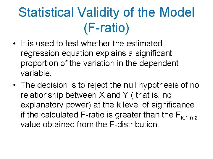
Statistical Validity of the Model (F-ratio) • It is used to test whether the estimated regression equation explains a significant proportion of the variation in the dependent variable. • The decision is to reject the null hypothesis of no relationship between X and Y ( that is, no explanatory power) at the k level of significance if the calculated F-ratio is greater than the Fk, 1, n-2 value obtained from the F-distribution.

Association and Causation • The presence of association (correlation) does not necessarily imply causation.

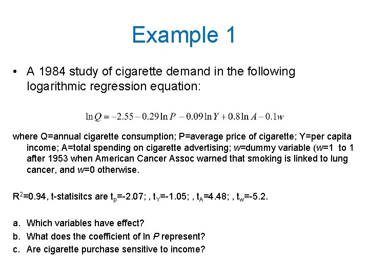
Example 1 • A 1984 study of cigarette demand in the following logarithmic regression equation: where Q=annual cigarette consumption; P=average price of cigarette; Y=per capita income; A=total spending on cigarette advertising; w=dummy variable (w=1 to 1 after 1953 when American Cancer Assoc warned that smoking is linked to lung cancer, and w=0 otherwise. R 2=0. 94, t-statisitcs are tp=-2. 07; , t. Y=-1. 05; , t. A=4. 48; , tw=-5. 2. a. Which variables have effect? b. What does the coefficient of ln P represent? c. Are cigarette purchase sensitive to income?

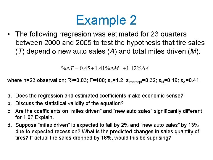
Example 2 • The following rregresion was estimated for 23 quarters between 2000 and 2005 to test the hypothesis that tire sales (T) depend o new auto sales (A) and total miles driven (M): where n=23 observation; R 2=0. 83; F=408; se=1. 2; sintercept=0. 32; s. M=0. 19; s. A=0. 41. a. Does the regression and estimated coefficients make economic sense? b. Discuss the statistical validity of the equation? c. Are the coefficients on “miles driven” and “new auto sales” significantly different for 1. 0? Explain. d. Suppose “miles driven” is expected to fall by 2% and “new auto sales” by 13% due to expected recession? What is the predicted changes in sales quantity of tires? If actual tire sales dropped by 18%, would this be suprising?

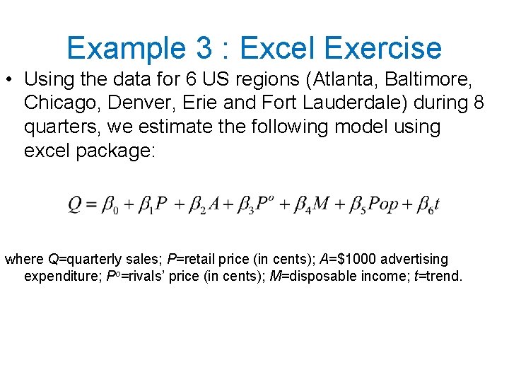
Example 3 : Excel Exercise • Using the data for 6 US regions (Atlanta, Baltimore, Chicago, Denver, Erie and Fort Lauderdale) during 8 quarters, we estimate the following model using excel package: where Q=quarterly sales; P=retail price (in cents); A=$1000 advertising expenditure; Po=rivals’ price (in cents); M=disposable income; t=trend.

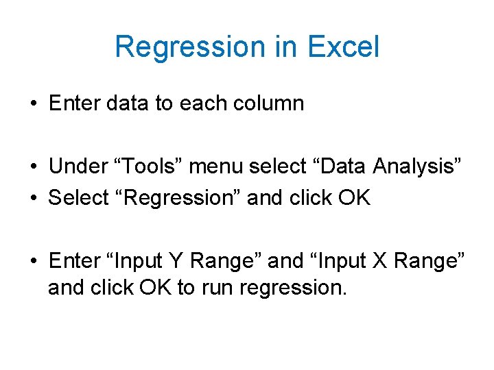
Regression in Excel • Enter data to each column • Under “Tools” menu select “Data Analysis” • Select “Regression” and click OK • Enter “Input Y Range” and “Input X Range” and click OK to run regression.

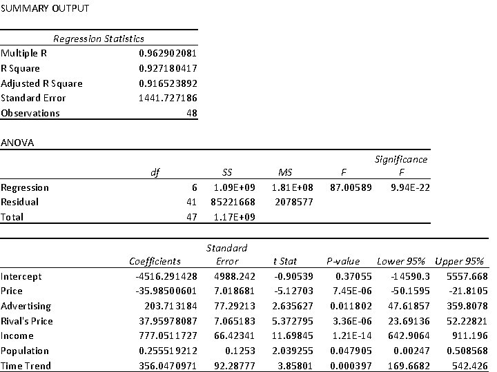
SUMMARY OUTPUT Regression Statistics Multiple R 0. 962902081 R Square 0. 927180417 Adjusted R Square 0. 916523892 Standard Error 1441. 727186 Observations 48 ANOVA Regression Residual Total 6 41 47 Intercept Price Advertising Rival's Price Income Population Time Trend df Coefficients -4516. 291428 -35. 98500601 203. 713184 37. 95978087 777. 0511727 0. 255519212 356. 0470971 SS 1. 09 E+09 85221668 1. 17 E+09 Standard Error 4988. 242 7. 018681 77. 29213 7. 065183 66. 42341 0. 1253 92. 28777 Significance F F 87. 00589 9. 94 E-22 MS 1. 81 E+08 2078577 t Stat -0. 90539 -5. 12703 2. 635627 5. 372795 11. 69845 2. 039255 3. 85801 P-value Lower 95% Upper 95% 0. 37055 -14590. 3 5557. 668 7. 45 E-06 -50. 1595 -21. 8105 0. 011802 47. 61857 359. 8078 3. 36 E-06 23. 69136 52. 22821 1. 21 E-14 642. 9064 911. 196 0. 047905 0. 00247 0. 508568 0. 000397 169. 6682 542. 426

Potential Problems in Regression • Equation Specification – Linear versus Nonlinear Models • Omitted Variables • Multicollinearity – Two or more explanatory variables are highly correlated • Autocorrelation – Error terms are highly correlated • Simultaneity and Identification