Changes to quantile mapping and weighting for PQPF

Changes to quantile mapping and weighting for PQPF using ECMWF reforecast data Tom Hamill, NOAA ESRL/PSD

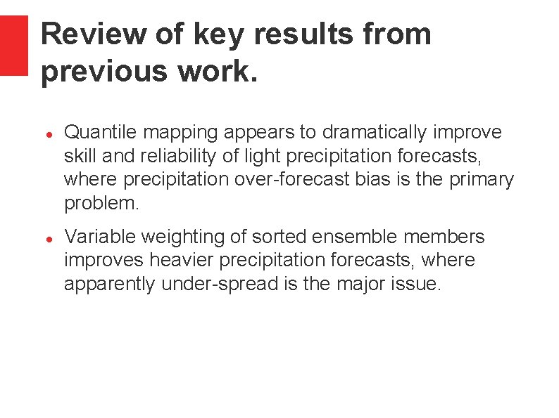
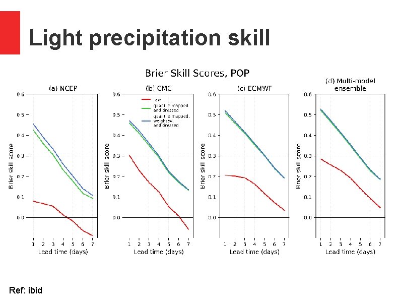
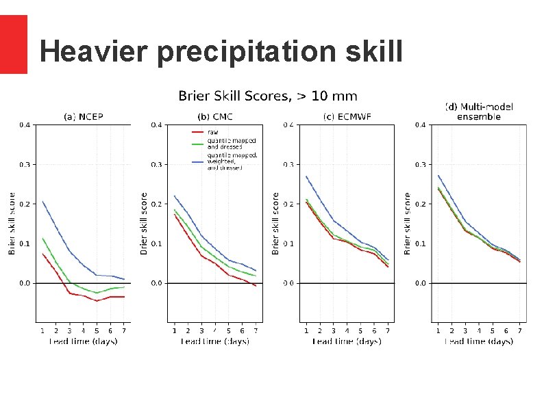
Review of key results from previous work. Quantile mapping appears to dramatically improve skill and reliability of light precipitation forecasts, where precipitation over-forecast bias is the primary problem. Variable weighting of sorted ensemble members improves heavier precipitation forecasts, where apparently under-spread is the major issue.

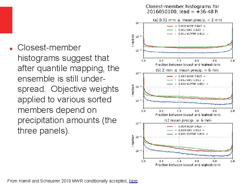
Closest-member histograms suggest that after quantile mapping, the ensemble is still underspread. Objective weights applied to various sorted members depend on precipitation amounts (the three panels). From Hamill and Scheuerer 2018 MWR conditionally accepted, here.

Light precipitation skill Ref: ibid

Heavier precipitation skill

Work completed Speeding up the quantile mapping code. New procedure for weighting ensemble to deal with the issue of varying ensemble size. Reforecast: 11 members. Real-time: 51 members. New procedure for synthetically generating a 51 member ensemble that are equally likely and preserve rank correlation structure of original ensemble.

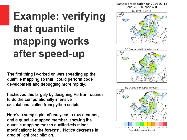
Example: verifying that quantile mapping works after speed-up The first thing I worked on was speeding up the quantile mapping so that I could perform code development and debugging more rapidly. I achieved this largely by designing Fortran routines to do the computationally intensive calculations, called from python scripts. Here’s a sample plot of analyzed, a raw member, and a quantile-mapped member, showing the quantile mapping makes qualitatively minor modifications to the forecast. Notice decrease in area of light precipitation.

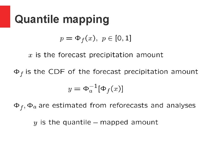
Determining closest-member histogram weights. Definition of these weights follows discussion in Hamill and Scheuerer (2018), here. Test data set of weights were accumulated over a set of 9 reforecast dates centered on 14 July, 20 years, and all grid points with valid data. A cross-validation procedure was applied, whereby: Vectors of weights were determined separately for light (0. 01 – 2. 0 mm) quantile-mapped ensemble-mean precipitation, moderate (2. 0 – 6. 0 mm), and heavy (> 6. 0 mm) For year i of m=20 years, the ith year of training data was withheld for determining the CDFs for quantile mapping. Then the quantile mapping was applied to that ith year with CDFs built using the remaining 19 years x 9 case days x 50 supplemental locations. I also fitted a Beta distribution and estimated weights from that, reason to be explained in next slides.

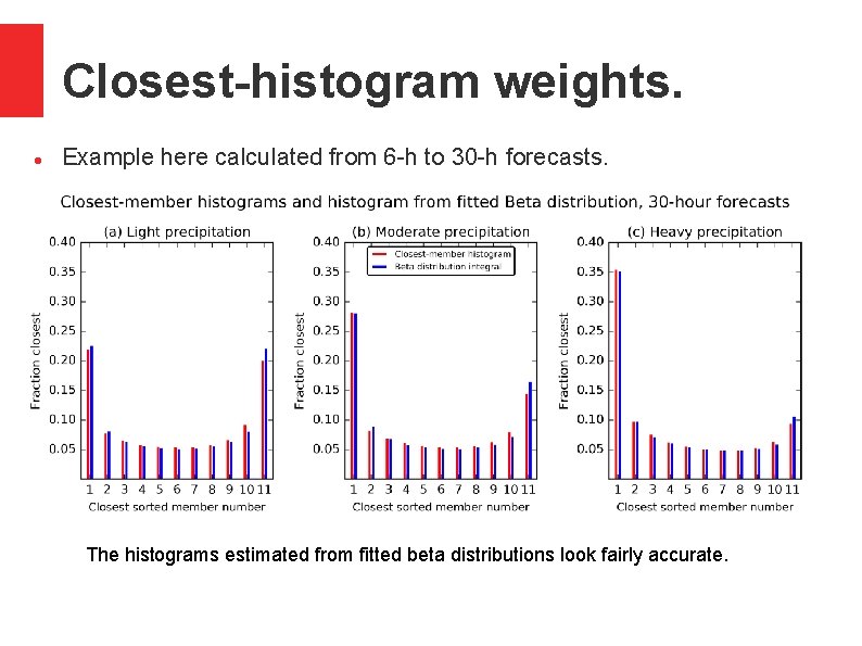
Closest-histogram weights. Example here calculated from 6 -h to 30 -h forecasts. The histograms estimated from fitted beta distributions look fairly accurate.

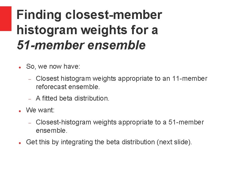
Finding closest-member histogram weights for a 51 -member ensemble So, we now have: Closest histogram weights appropriate to an 11 -member reforecast ensemble. A fitted beta distribution. We want: Closest-histogram weights appropriate to a 51 -member ensemble. Get this by integrating the beta distribution (next slide).

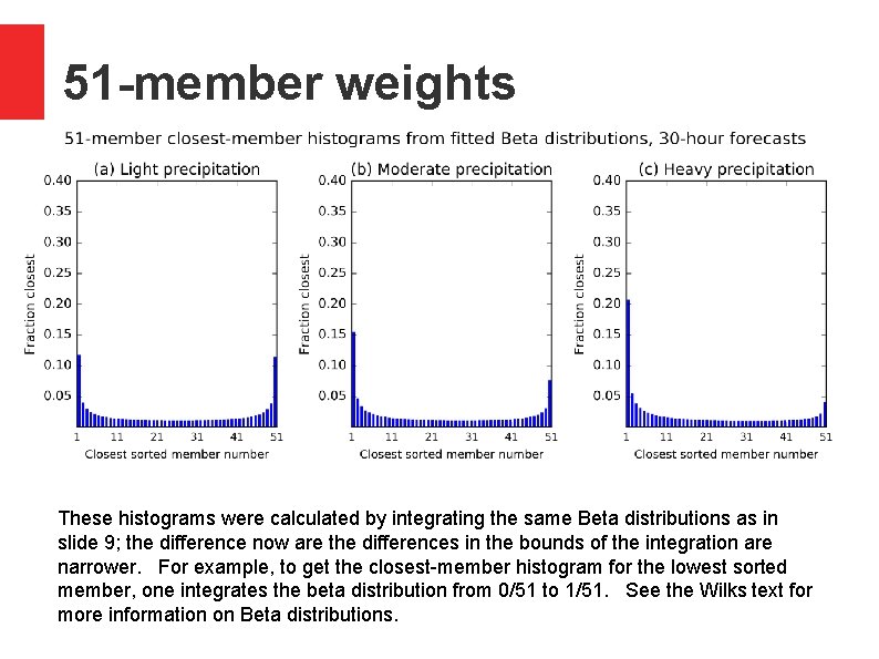
51 -member weights These histograms were calculated by integrating the same Beta distributions as in slide 9; the difference now are the differences in the bounds of the integration are narrower. For example, to get the closest-member histogram for the lowest sorted member, one integrates the beta distribution from 0/51 to 1/51. See the Wilks text for more information on Beta distributions.

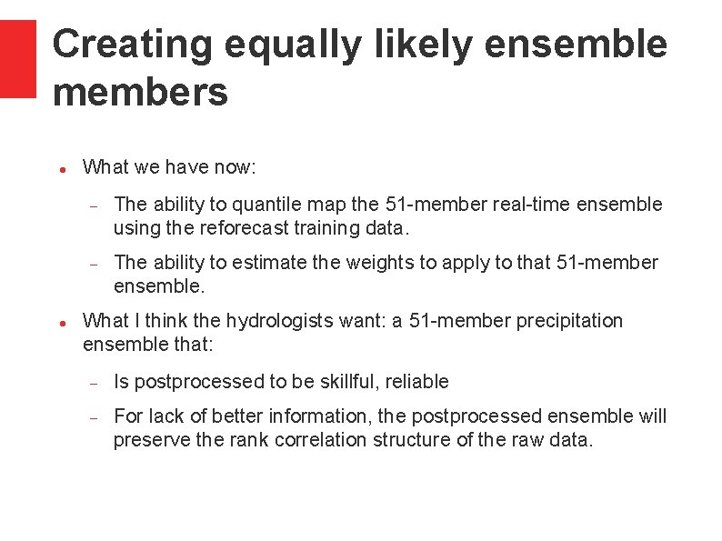
Creating equally likely ensemble members What we have now: The ability to quantile map the 51 -member real-time ensemble using the reforecast training data. The ability to estimate the weights to apply to that 51 -member ensemble. What I think the hydrologists want: a 51 -member precipitation ensemble that: Is postprocessed to be skillful, reliable For lack of better information, the postprocessed ensemble will preserve the rank correlation structure of the raw data.

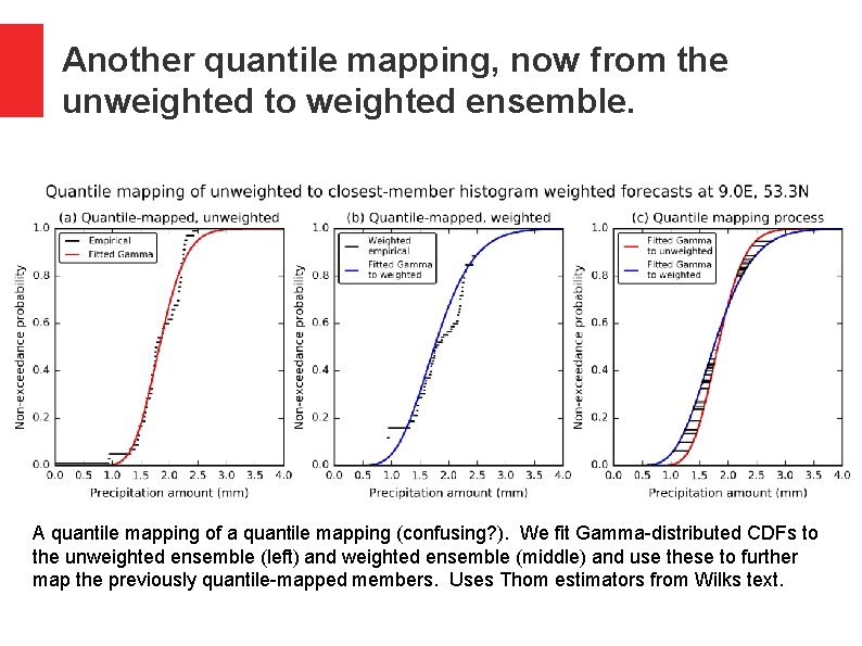
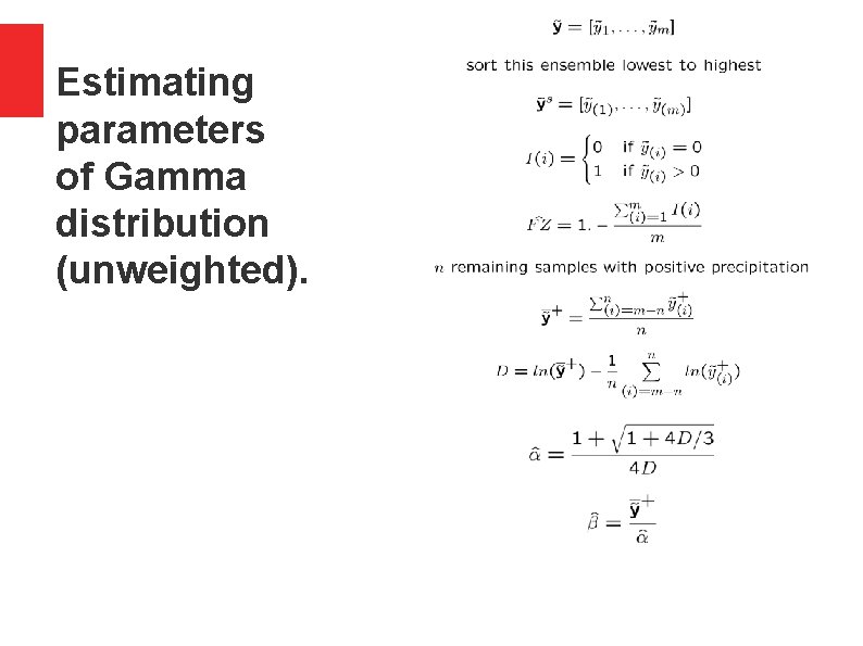
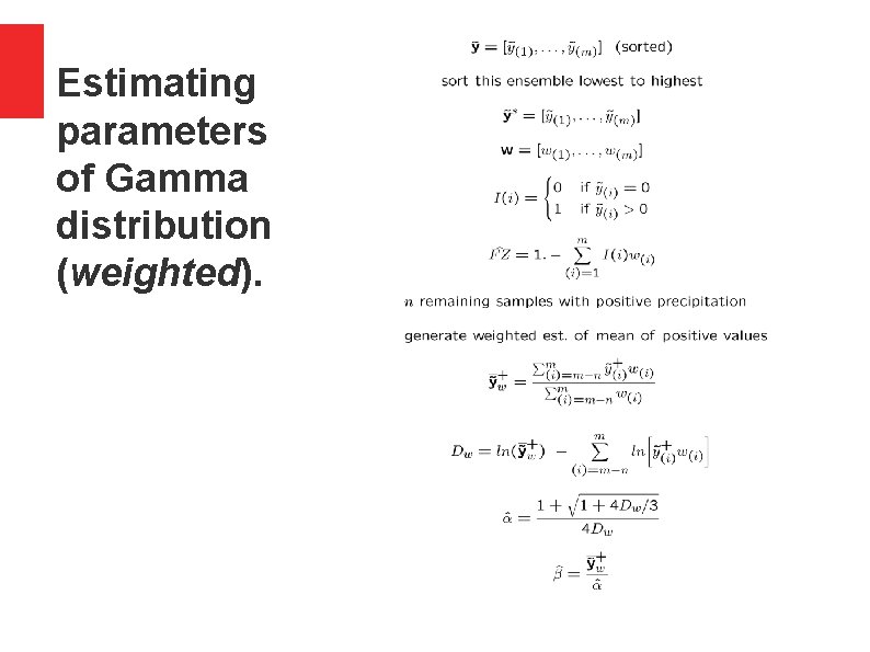
Another quantile mapping, now from the unweighted to weighted ensemble. A quantile mapping of a quantile mapping (confusing? ). We fit Gamma-distributed CDFs to the unweighted ensemble (left) and weighted ensemble (middle) and use these to further map the previously quantile-mapped members. Uses Thom estimators from Wilks text.

Estimating parameters of Gamma distribution (unweighted).

Estimating parameters of Gamma distribution (weighted).

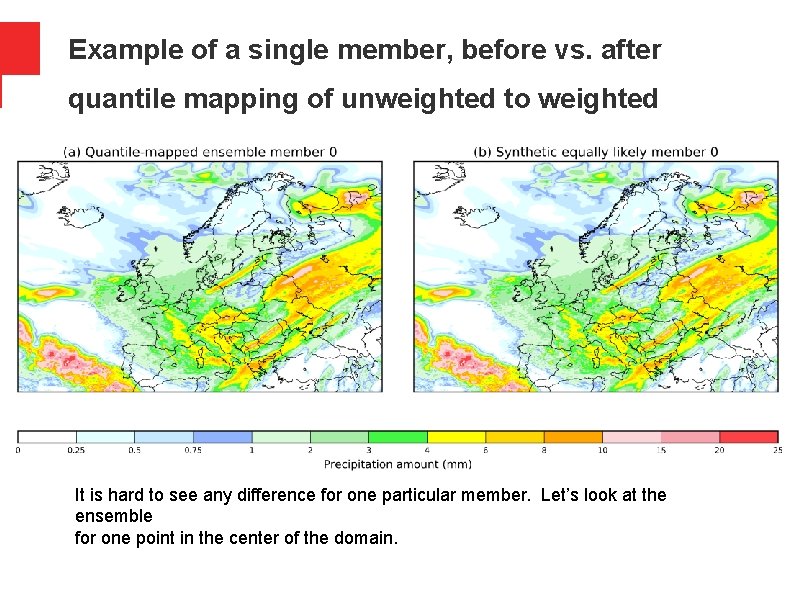
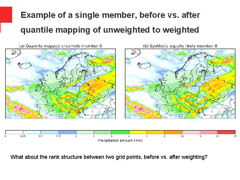
Example of a single member, before vs. after quantile mapping of unweighted to weighted It is hard to see any difference for one particular member. Let’s look at the ensemble for one point in the center of the domain.

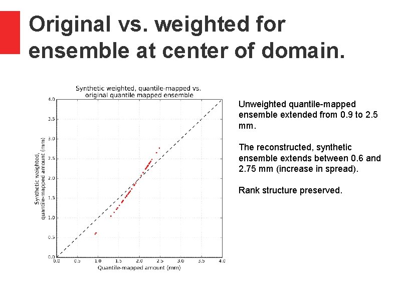
Original vs. weighted for ensemble at center of domain. Unweighted quantile-mapped ensemble extended from 0. 9 to 2. 5 mm. The reconstructed, synthetic ensemble extends between 0. 6 and 2. 75 mm (increase in spread). Rank structure preserved.

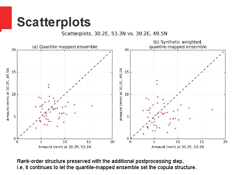
Example of a single member, before vs. after quantile mapping of unweighted to weighted What about the rank structure between two grid points, before vs. after weighting?

Scatterplots Rank-order structure preserved with the additional postprocessing step, i. e, it continues to let the quantile-mapped ensemble set the copula structure.

Conclusions I think I have some code elements that can be adapted to provide high-quality post-processed precipitation ensembles to drive EFAS. Any further work you’d like to see me complete before my departure? Will try to continue to help from Boulder, but obviously much easier now.

Quantile mapping