WARM UP As an employee of Pizza Hut

WARM – UP As an employee of Pizza Hut, your boss has put you in charge of determining the likeability of a New kind of Pizza. Using the 6 W’s, how would you precede? Be detailed!!!

WARM – UP Your boss has put you in charge of developing a new version of the popular video game “HALO” Describe The W’s of Data Collection and Analysis : Who, What, Why, When, Where, and Ho. W.

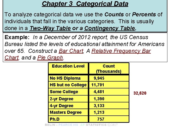
Chapter 3 Categorical Data To analyze categorical data we use the Counts or Percents of individuals that fall in the various categories. This is usually done in a Two-Way Table or a Contingency Table. Example: In a December of 2012 report, the US Census Bureau listed the levels of educational attainment for Americans over 65. Construct a Bar Chart, A Relative Frequency Bar Chart, and a Pie Graph. Education Level No HS Diploma HS but no College Count (Thousands) 9, 945 11, 701 Some College 4, 481 2 -yr Degree 1, 390 4 -yr Degree 3, 133 Masters Degree 1, 213 Ph. D 757 32, 620

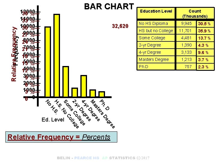
Relative Frequency 32, 620 Education Level Count (Thousands) No HS Diploma 9, 945 30. 5 % 11, 701 35. 9 % Some College 4, 481 13. 7 % 2 -yr Degree 1, 390 4. 3 % 4 -yr Degree 3, 133 9. 6 % Masters Degree 1, 213 3. 7 % 757 2. 3 % HS but no College Ph. D ee gr. D De Ph ers e t as gre M De e yr gre e 4 De leg e yr ol 2 - e C lleg m Co So No S. H. No 12000— 36 %— 11000— 33 %— 10000— 30 %— 9000— 27 %— 8000— 24 %— 7000— 21 %— 6000— 18 %— 5000— 15 %— 4000— 12 %— 3000— 9 %— 2000— 6 %— 1000— 3 %— 0 0— BAR CHART Ed. Level Relative Frequency = Percents

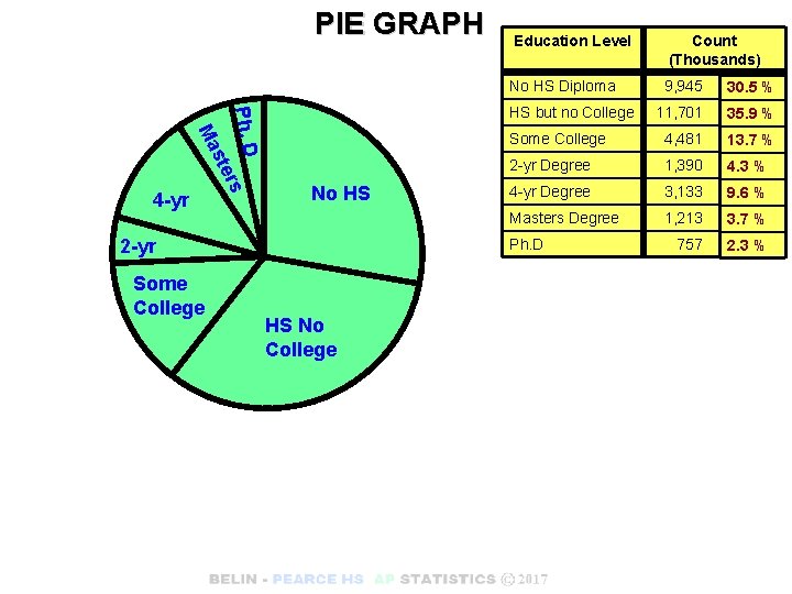
PIE GRAPH Ph. D rs No HS 2 -yr Some College Count (Thousands) No HS Diploma 9, 945 30. 5 % 11, 701 35. 9 % Some College 4, 481 13. 7 % 2 -yr Degree 1, 390 4. 3 % 4 -yr Degree 3, 133 9. 6 % Masters Degree 1, 213 3. 7 % 757 2. 3 % HS but no College ste Ma 4 -yr Education Level Ph. D HS No College

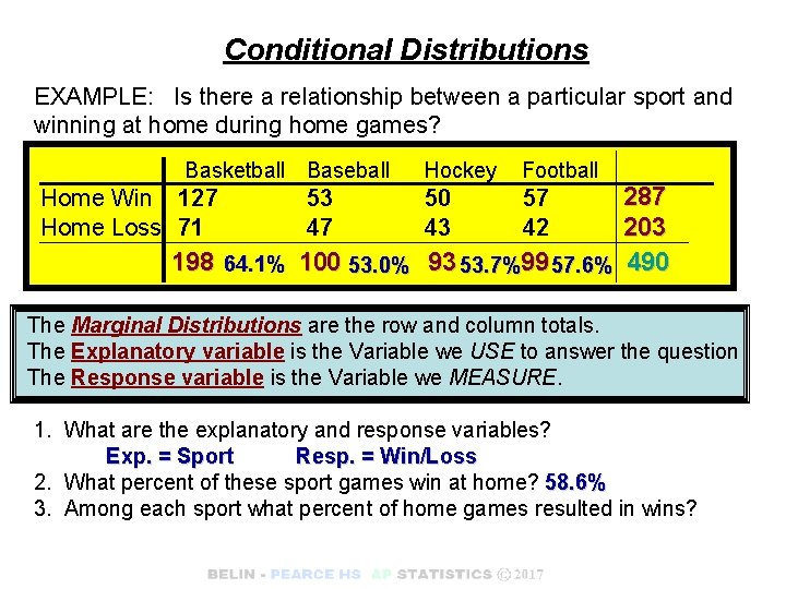
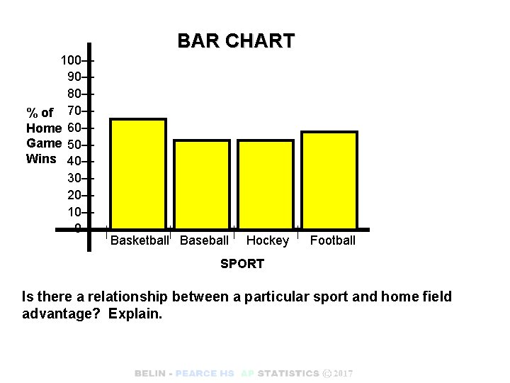
Conditional Distributions EXAMPLE: Is there a relationship between a particular sport and winning at home during home games? Basketball Baseball Home Win 127 Home Loss 71 198 64. 1% 53 47 100 53. 0% Hockey Football 50 57 43 42 93 53. 7%99 57. 6% 287 203 490 The Marginal Distributions are the row and column totals. The Explanatory variable is the Variable we USE to answer the question The Response variable is the Variable we MEASURE. 1. What are the explanatory and response variables? Exp. = Sport Resp. = Win/Loss 2. What percent of these sport games win at home? 58. 6% 3. Among each sport what percent of home games resulted in wins?

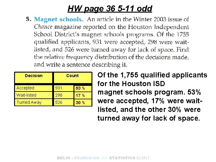
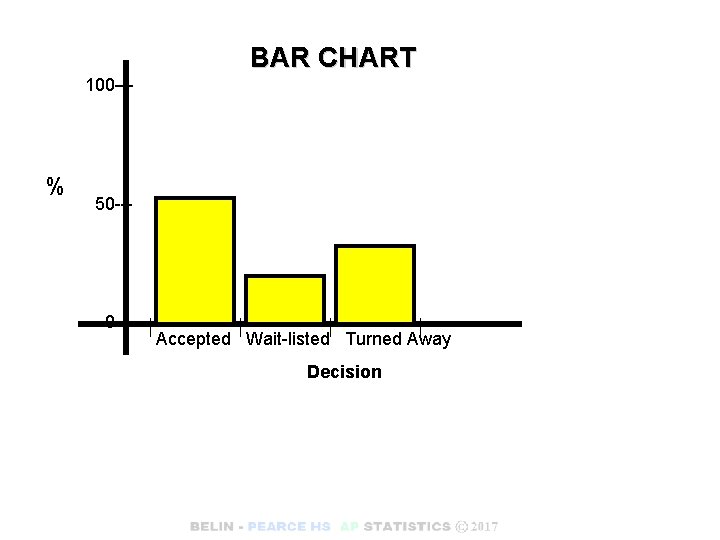
HW page 36 5 -11 odd Decision Count Accepted 931 53 % Wait-listed 298 17 % Turned Away 526 30 % Of the 1, 755 qualified applicants for the Houston ISD magnet schools program. 53% were accepted, 17% were waitlisted, and the other 30% were turned away for lack of space.

BAR CHART 100— % 50 --- 0— Accepted Wait-listed Turned Away Decision

BAR CHART 100— 90— 80— % of 70— Home 60— Game 50— Wins 40— 30— 20— 10— 0— Basketball Baseball Hockey Football SPORT Is there a relationship between a particular sport and home field advantage? Explain.