Scaling Up n Integrating Smaller Scale RestorationModelingMonitoring Projects

Scaling Up n Integrating Smaller Scale Restoration/Modeling/Monitoring Projects with the Chesapeake Bay Watershed Model

To Scale or Not to Scale n Can information from Targeted watershed monitoring and modeling projects be useful in a watershed scale module like the CBWM? n n Yes, if we can gather good information, and if we model the processes that are embodied by the newest BMPs: n n Admittedly, some of these projects are far from “small”. What are the nitty-gritty details of BMPs? What information about those BMPs is useful? What processes are scalable, what are not? To answer these questions, we also need to know the input demands and processes represented in the CBWM

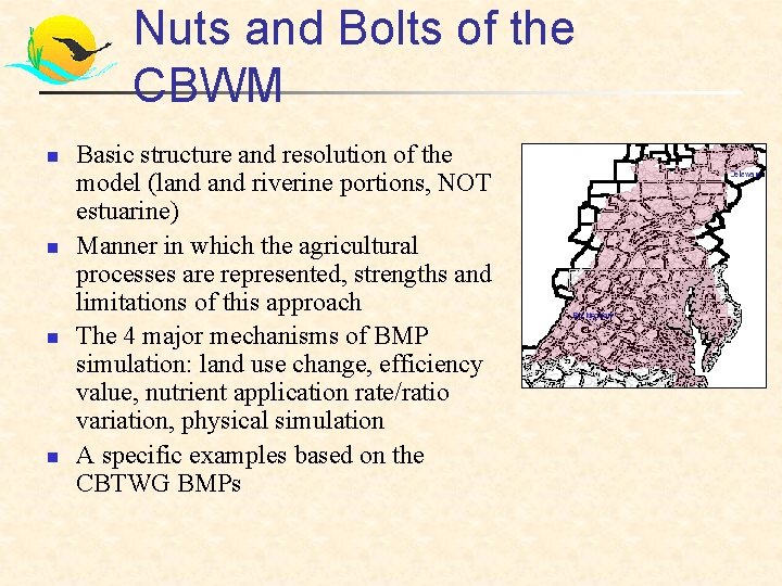
Nuts and Bolts of the CBWM n n Basic structure and resolution of the model (land riverine portions, NOT estuarine) Manner in which the agricultural processes are represented, strengths and limitations of this approach The 4 major mechanisms of BMP simulation: land use change, efficiency value, nutrient application rate/ratio variation, physical simulation A specific examples based on the CBTWG BMPs

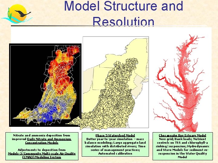
Model Structure and Resolution Nitrate and ammonia deposition from improved Daily Nitrate and Ammonium Concentration Models Adjustments to deposition from Models-3/Community Multi-scale Air Quality (CMAQ) Modeling System Phase 5 Watershed Model Better year-to-year simulation – mass balance modeling; Large aggregate land simulation with distributed rivers; Time series of management practices; Automated calibration Chesapeake Bay Estuary Model New grid; Bank loads; Nutrient controls on TSS and chlorophyll-a sinking/suspension; Hydrodynamic and Wave Models for sediment resuspension in the Water Quality Model

Model Structure and Resolution (cont. ) n Based on Enhanced HSPF code n n 26 land-uses per segment n n n 16 ag, 5 urban, mining, forest, grass/meadow, water Resolution: n n 1 hour time-step, 15 minutes in one small basin 1, 064 individual reaches 2, 365 land/river segment 61, 490 individual moving parts Average lu/lrseg ≈ 1, 000 acres Inputs are atmospheric, fertilizer legume, point source, septic Spatial distribution is obtained by: n n Smaller model segments give implicit spatial context Varying hydrologic and NPS parameters by land use In-stream linkage is implicitly spatial HSPF allows series routing of land-uses, example: buffers

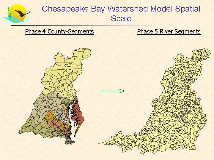
Chesapeake Bay Watershed Model Spatial Scale Phase 4 County-Segments Phase 5 River Segments

Agricultural Simulation n 16 Ag Land-uses: n n Vary by tillage, crop type, fertilizer rate (nutrient management), presence of livestock Uses the AGCHEM module of HSPF n Yield-based algorithm n n n Maximum uptake / return to soil “Composite Crop” – single crop per year Application timing, amounts based on crop type, fertilizer type Uptake, applications, are “quasi-monthly” (trapezoidal) Manure is applied in county in which it is generated, unless we are told otherwise

Agricultural Model: Model Goals n Realistically Model Agricultural Lands: n n n Long-term soil nutrient balances Nutrient mineralization rates Crop Uptake Effects of drought and nutrient wash-off Reaction to varying nutrient sources

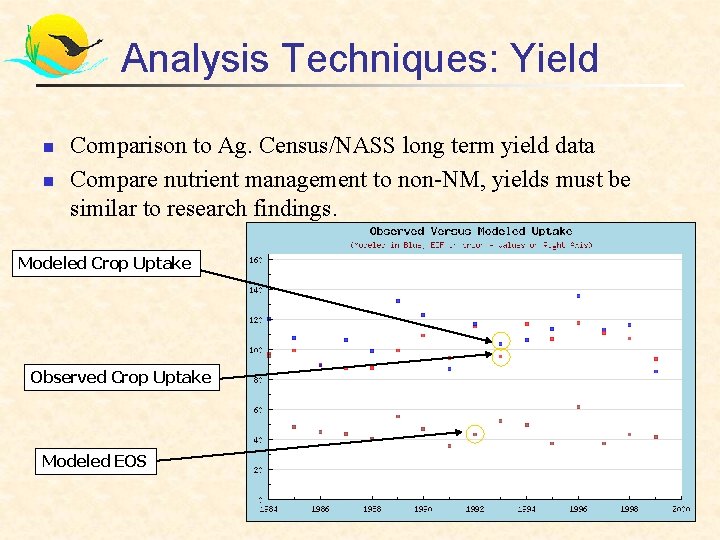
Analysis Techniques: Yield n n Comparison to Ag. Census/NASS long term yield data Compare nutrient management to non-NM, yields must be similar to research findings. Modeled Crop Uptake Observed Crop Uptake Modeled EOS

BMP Simulation n n n Efficiency: edge of field output is multiplied by some reduction factor before delivery to the stream. Land Use Change: Acres are converted from one modeled land use to another to represent the BMP. Altered Inputs: Change amount, timing, or type of nutrient inputs. Model is remarkably sensitive to timing. Physical simulation: alter physical characteristics such as roughness, infiltration, or other (really, more a sub-category of land-use change). Advanced Physical Sim. : Route runoff from upland-uses through a buffer strip land-use (permissible in HSPF 12) Note: Physical simulation, Altered Inputs or Lu Change are preferable if your land use is understood, fits into model framework, and is well calibrated

Simulation of CBTWG BMPs n n Forest Buffers, efficiency + LU Change – 1 acre treats 4 acres of upland runoff, reducing N (22 -75%), P (42 -68%), and S(4268%). Land converted to forest. Continuous no-till, LU Change + Efficiency: High till goes to low-till – low-till land use has a higher infiltration, roughness, lower nutrient yield. Nutrient management, Altered Inputs – NM land use is the same as as parent land use (including soil reactions), but lower application rate. Drainage Control, Physical Simulation/effic. : Could alter the Reach output curve (FTABLE) to mimic detention, nitrogen transformations. Big question: what are relative contributions of de-nitrification and enhanced nutrient uptake efficiency. Currently, it is an efficiency.

CBTWG BMPs (continued) n n n Cover Crops, efficiency/physical: We currently model cover crops as an efficiency, but we model winter small grains physically. If we know the relevant information about the cover crops, uptake timing, amount, limiting factors, we can physically model them. Non-structural Stormwater control, efficiency/lu-change: Land converted to forest, wetlands as efficiency, effects of stream restoration? Trading Programs, altered inputs: Similar to nutrient management, we physically move the nutrients from one place in the model to another, but perhaps this will take the application reductions to a new level?

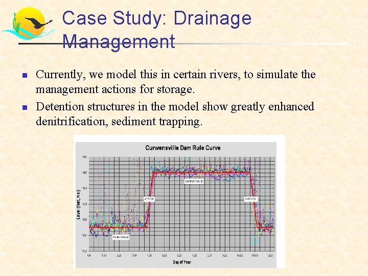
Case Study: Drainage Management n n Currently, we model this in certain rivers, to simulate the management actions for storage. Detention structures in the model show greatly enhanced denitrification, sediment trapping.

Case Study: Cover Crops n Currently Simulated as an Efficiency: n n Reduction N (30%), P(10%), S(10%) Same reduction every year Applied across the entire years EOS load Alternative Approach: Model using the AGCHEM module n n Need monthly uptake of nutrients by cover crops as monitored in the field Maximum Uptake possible (theoretical max) n n Effect of planting date on total uptake potential n n n This varies by location and variety planted, is this data recorded in ongoing studies? What factors govern this? Frost? Max daily temperature? Other? Data on how the total uptake of a cover crop is affected by moisture/drought Already doing small grains, fall/spring uptake curves, nutrient applications (or not)

Case Study: CNT n n Currently modeled as low till + Efficiency Questions remain: n n Does the increased nitrogen retention from OM build-up persist in perpetuity, or is it reduced after some time period? Does dissolved P increase? Can we simulate this accurately?

Conclusion n Can We Learn Important Things From Smaller Scale Studies? n n n Absolutely, what data do these projects have that we don’t already know about? What situations are un-clear to our current models, i. e. , what can’t we model? What are we missing in terms of the major mechanisms? Are there new land uses, or improved understanding of current land use behaviors that our models can implement? Are there things that will not scale up?