Physical Oceanography Mass is conserved density measurements massvolume

Physical Oceanography: • Mass is conserved – density measurements (mass/volume) • Momentum* is conserved – velocity measurements (*) momentum=mass*velocity

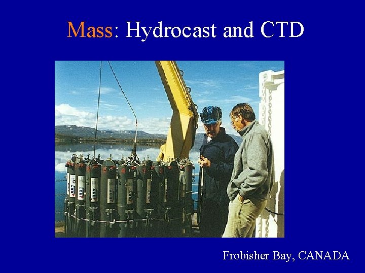
Mass: Hydrocast and CTD Frobisher Bay, CANADA

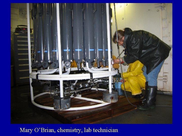
Mary O’Brian, chemistry, lab technician

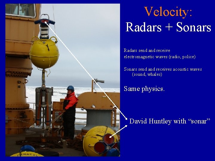
Velocity: Radars + Sonars Radars send and receive electromagnetic waves (radio, police) Sonars send and receives acoustic waves (sound, whales) Same physics. David Huntley with “sonar”

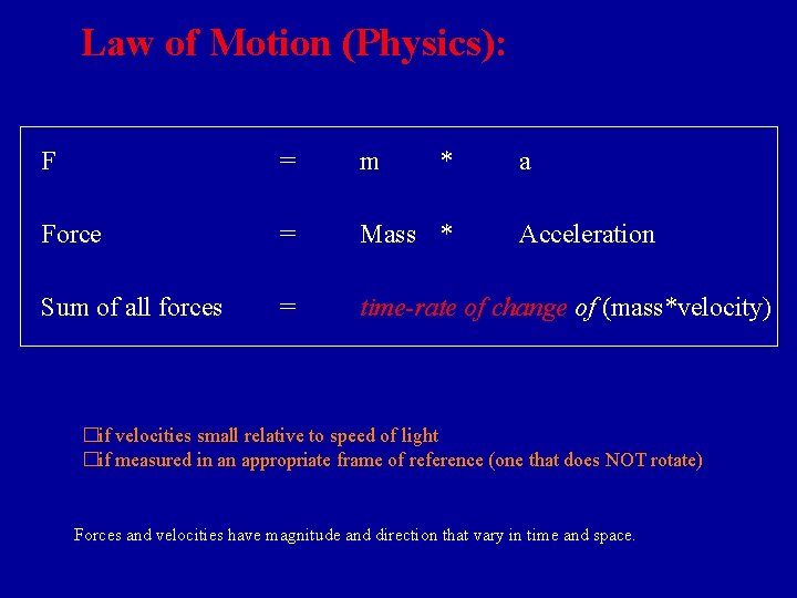
Law of Motion (Physics): F = m * a Force = Mass * Sum of all forces = time-rate of change of (mass*velocity) Acceleration �if velocities small relative to speed of light �if measured in an appropriate frame of reference (one that does NOT rotate) Forces and velocities have magnitude and direction that vary in time and space.

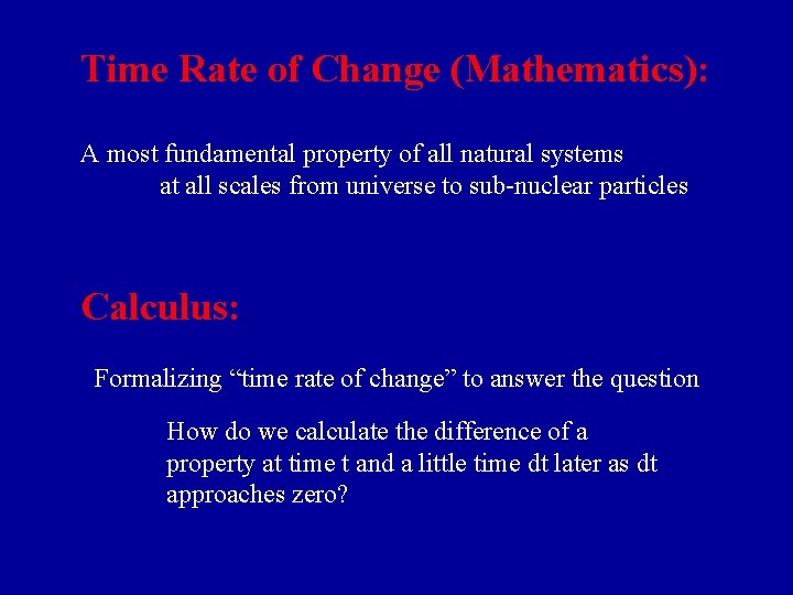
Time Rate of Change (Mathematics): A most fundamental property of all natural systems at all scales from universe to sub-nuclear particles Calculus: Formalizing “time rate of change” to answer the question How do we calculate the difference of a property at time t and a little time dt later as dt approaches zero?

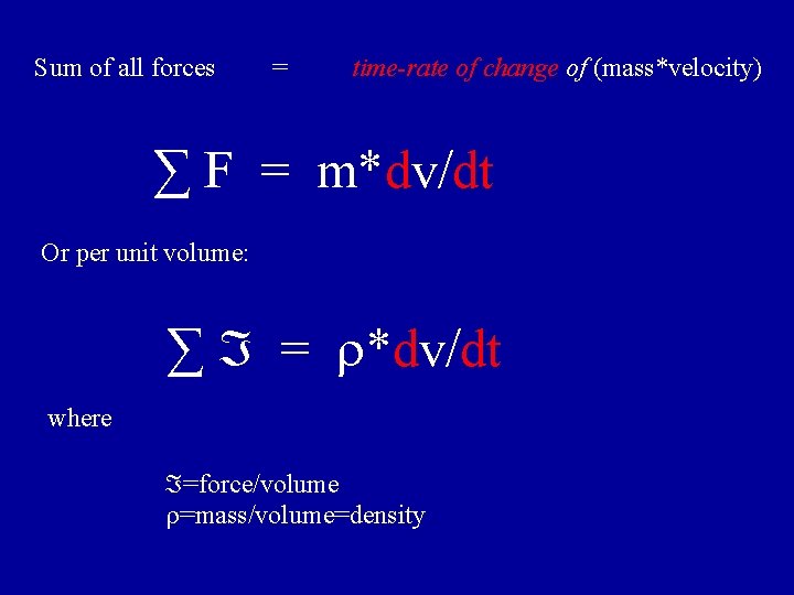
Sum of all forces = time-rate of change of (mass*velocity) ∑ F = m*dv/dt Or per unit volume: ∑ = *dv/dt where =force/volume =mass/volume=density

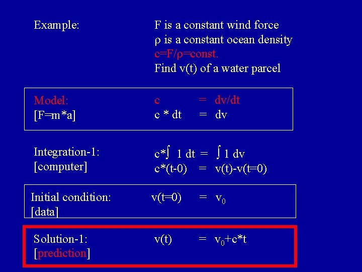
Example: F is a constant wind force is a constant ocean density c=F/ =const. Find v(t) of a water parcel Model: [F=m*a] c c * dt Integration-1: [computer] c*∫ 1 dt = ∫ 1 dv c*(t-0) = v(t)-v(t=0) Initial condition: [data] v(t=0) = v 0 Solution-1: [prediction] v(t) = v 0+c*t = dv/dt = dv

Solution-1: v(t) = v 0 + c*t Recall: v = dx/dt Integration-2: [computer] v*dt = dx ∫ v(t) dt = ∫ 1 dx ∫ (v 0 + c*t) dt = ∫ 1 dx v 0*t + c*t 2/2 = x(t)-x(t=0) Initial condition: [Data] x(t=0) = x 0 Solution-2: [Prediction] x(t) = x 0 + v 0*t + c*t 2/2

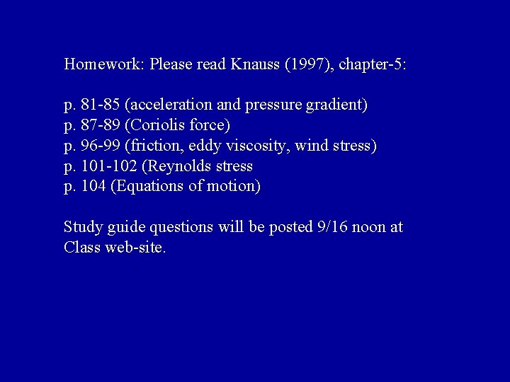
Homework: Please read Knauss (1997), chapter-5: p. 81 -85 (acceleration and pressure gradient) p. 87 -89 (Coriolis force) p. 96 -99 (friction, eddy viscosity, wind stress) p. 101 -102 (Reynolds stress p. 104 (Equations of motion) Study guide questions will be posted 9/16 noon at Class web-site.