Operations Research I MCNF Network Simplex Instructors Martin

Operations Research I: MCNF & Network Simplex Instructors: Martin Savelsbergh & Masoud Talebian

Minimum Cost Network Flow Problems n includes assignment, transportation, maximum flow, CPM, and shortest path as special cases n Has a constraint matrix that is the node arc incidence matrix n Has integer valued solutions when solved by simplex n All are efficiently solvable

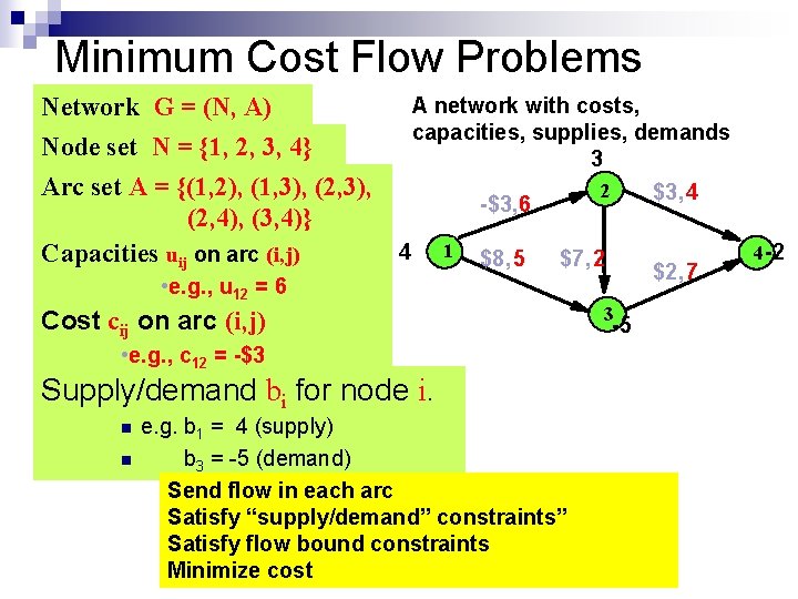
Minimum Cost Flow Problems Network G = (N, A) Node set N = {1, 2, 3, 4} Arc set A = {(1, 2), (1, 3), (2, 4), (3, 4)} 4 Capacities uij on arc (i, j) A network with costs, capacities, supplies, demands 3 2 $3, 4 -$3, 6 1 $8, 5 $7, 2 • e. g. , u 12 = 6 Cost cij on arc (i, j) • e. g. , c 12 = -$3 Supply/demand bi for node i. n n e. g. b 1 = 4 (supply) b 3 = -5 (demand) Send flow in each arc Satisfy “supply/demand” constraints” Satisfy flow bound constraints Minimize cost $2, 7 3 -5 4 -2

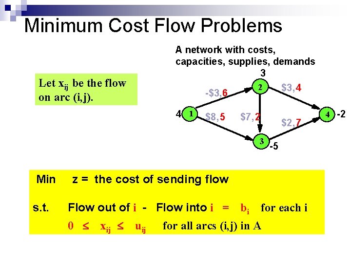
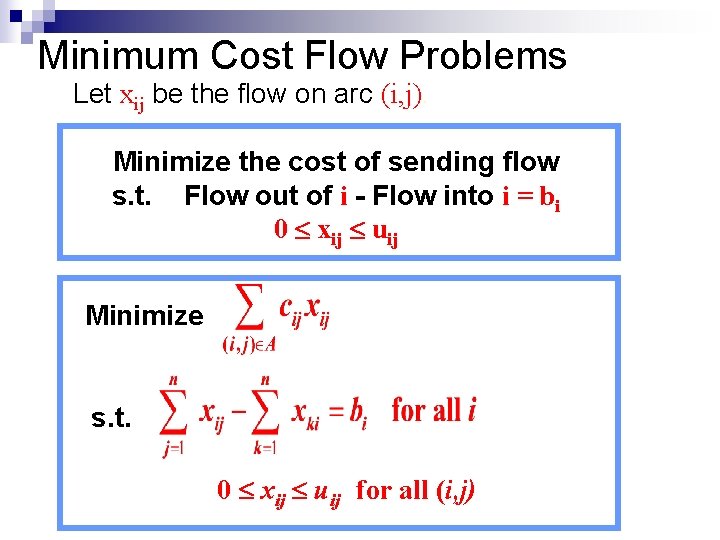
Minimum Cost Flow Problems A network with costs, capacities, supplies, demands 3 Let xij be the flow on arc (i, j). -$3, 6 4 1 $8, 5 2 $7, 2 3 Min s. t. $3, 4 $2, 7 -5 z = the cost of sending flow Flow out of i - Flow into i = 0 xij uij bi for each i for all arcs (i, j) in A 4 -2

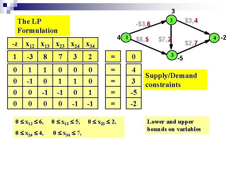
3 The LP Formulation -$3, 6 4 1 $8, 5 -z x 12 x 13 x 24 x 34 1 -3 8 7 3 2 = 0 0 0 1 -1 1 0 0 = = 4 3 0 0 -1 1 -1 = = -5 -2 0 x 12 6, 0 x 13 5, 0 x 24 4, 0 x 34 7, 0 x 23 2, 2 $3, 4 $7, 2 3 $2, 7 -5 Supply/Demand constraints Lower and upper bounds on variables 4 -2

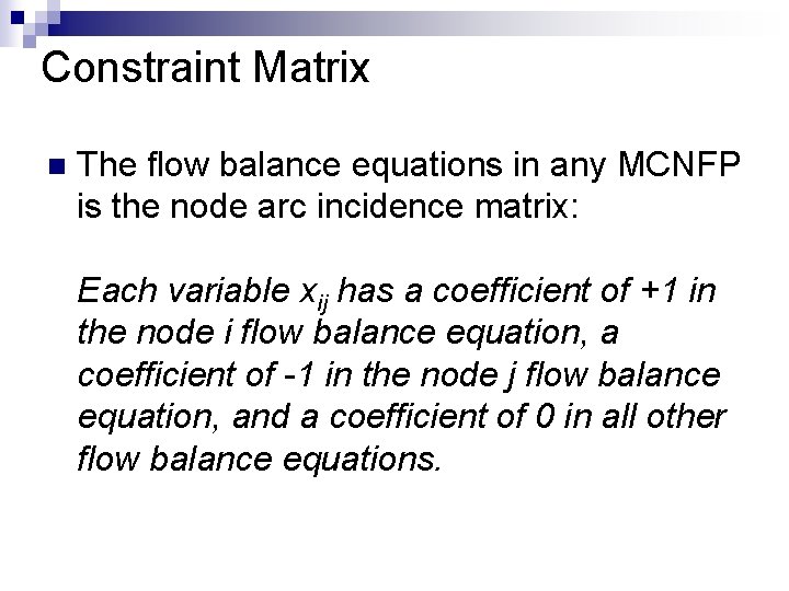
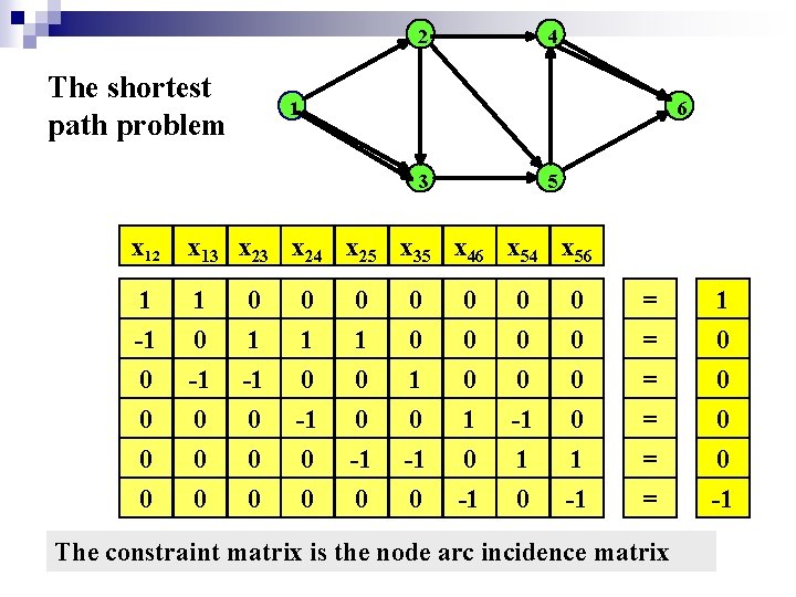
Constraint Matrix n The flow balance equations in any MCNFP is the node arc incidence matrix: Each variable xij has a coefficient of +1 in the node i flow balance equation, a coefficient of -1 in the node j flow balance equation, and a coefficient of 0 in all other flow balance equations.

Minimum Cost Flow Problems Let xij be the flow on arc (i, j). Minimize the cost of sending flow s. t. Flow out of i - Flow into i = bi 0 xij uij Minimize s. t. 0 xij uij for all (i, j)

Minimum Cost Flow Problems Upper bound constraints on variables may be treated similarly to lower bound constraints, and are not viewed as part of the constraint matrix.

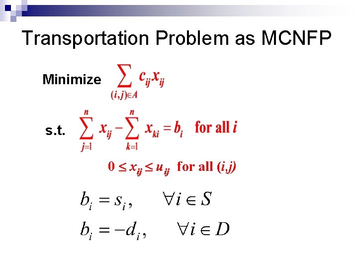
Transportation Problem as MCNFP Minimize s. t. 0 xij uij for all (i, j)

2 The shortest path problem 4 1 6 3 5 x 12 x 13 x 24 x 25 x 35 x 46 x 54 x 56 1 1 0 0 0 0 = 1 -1 0 0 0 1 0 -1 0 0 0 1 0 -1 0 0 -1 1 0 0 1 -1 = = = 0 0 -1 The constraint matrix is the node arc incidence matrix

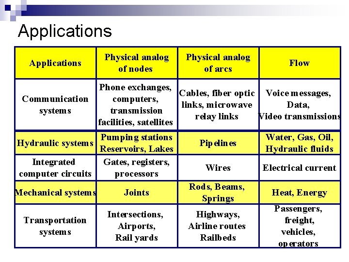
Applications Physical analog of nodes Physical analog of arcs Flow Phone exchanges, Cables, fiber optic Voice messages, Communication computers, links, microwave Data, systems transmission relay links Video transmissions facilities, satellites Pumping stations Reservoirs, Lakes Integrated Gates, registers, computer circuits processors Hydraulic systems Pipelines Water, Gas, Oil, Hydraulic fluids Wires Electrical current Heat, Energy Mechanical systems Joints Rods, Beams, Springs Transportation systems Intersections, Airports, Rail yards Highways, Airline routes Railbeds Passengers, freight, vehicles, operators

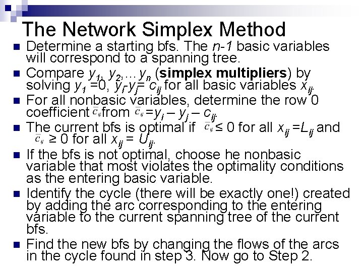
The Network Simplex Method n n n n Determine a starting bfs. The n-1 basic variables will correspond to a spanning tree. Compare y 1, y 2, …yn (simplex multipliers) by solving y 1 =0, yi-yj= cij for all basic variables xij. For all nonbasic variables, determine the row 0 coefficient from =yi – yj – cij. The current bfs is optimal if ≤ 0 for all xij =Lij and ≥ 0 for all xij = Uij. If the bfs is not optimal, choose he nonbasic variable that most violates the optimality conditions as the entering basic variable. Identify the cycle (there will be exactly one!) created by adding the arc corresponding to the entering variable to the current spanning tree of the current bfs. Find the new bfs by changing the flows of the arcs in the cycle found in step 3. Now go to Step 2.