Image enhancement in the spatial domain Human vision

Image enhancement in the spatial domain

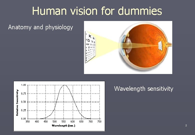
Human vision for dummies Anatomy and physiology Wavelength sensitivity 2

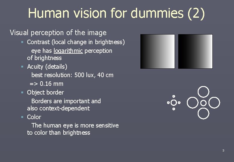
Human vision for dummies (2) Visual perception of the image § Contrast (local change in brightness) eye has logarithmic perception of brightness § Acuity (details) best resolution: 500 lux, 40 cm => 0. 16 mm § Object border Borders are important and also context-dependent § Color The human eye is more sensitive to color than brightness 3

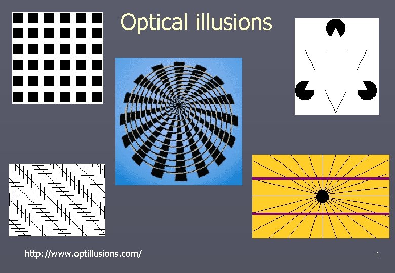
Optical illusions http: //www. optillusions. com/ 4

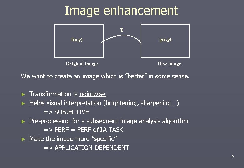
Image enhancement T f(x, y) Original image g(x, y) New image We want to create an image which is ”better” in some sense. ► ► Transformation is pointwise Helps visual interpretation (brightening, sharpening…) => SUBJECTIVE Pre-processing for a subsequent image analysis algorithm => PERF = PERF of IA TASK Make the image more ”specific” => APPLICATION DEPENDENT 5

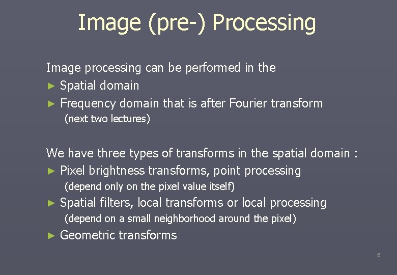
Image (pre-) Processing Image processing can be performed in the ► Spatial domain ► Frequency domain that is after Fourier transform (next two lectures) We have three types of transforms in the spatial domain : ► Pixel brightness transforms, point processing (depend only on the pixel value itself) ► Spatial filters, local transforms or local processing (depend on a small neighborhood around the pixel) ► Geometric transforms 6

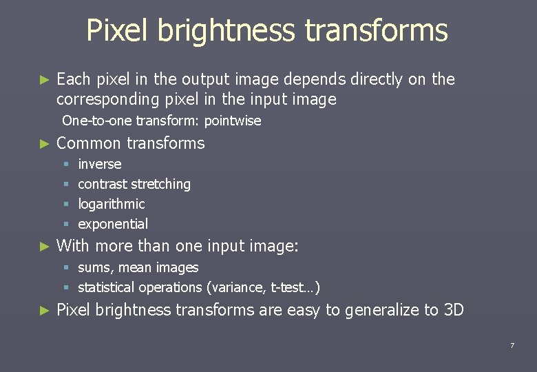
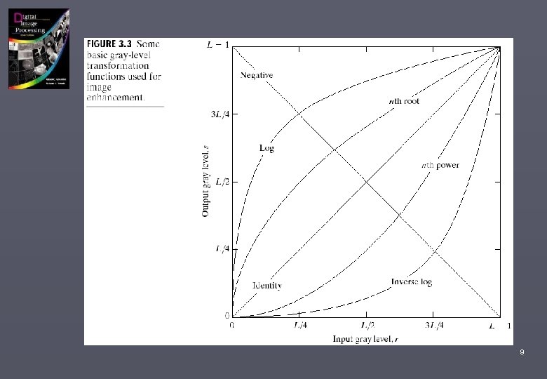
Pixel brightness transforms ► Each pixel in the output image depends directly on the corresponding pixel in the input image One-to-one transform: pointwise ► Common transforms § § ► inverse contrast stretching logarithmic exponential With more than one input image: § sums, mean images § statistical operations (variance, t-test…) ► Pixel brightness transforms are easy to generalize to 3 D 7

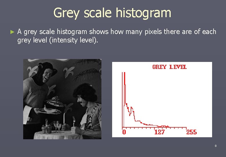
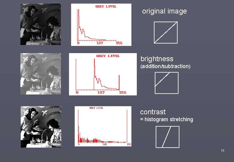
Grey scale histogram ► A grey scale histogram shows how many pixels there are of each grey level (intensity level). 8

9

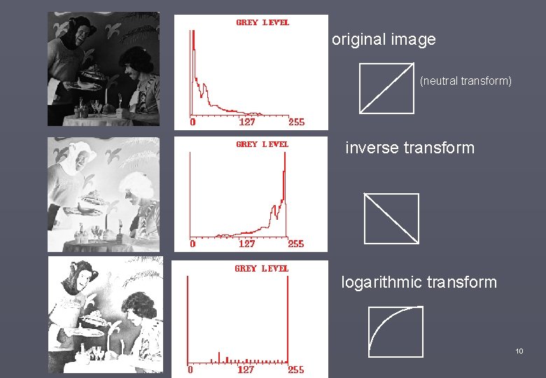
original image (neutral transform) inverse transform logarithmic transform 10

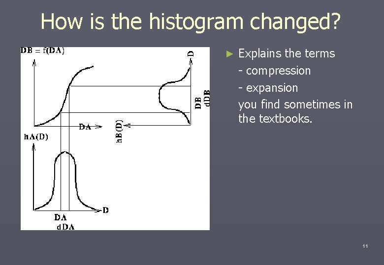
How is the histogram changed? ► Explains the terms - compression - expansion you find sometimes in the textbooks. 11

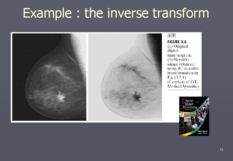
Example : the inverse transform 12

original image brightness (addition/subtraction) contrast = histogram stretching 13

Paint Shop Pro example What do the function do? ► How to use them to get the best results? And why it is best. ► ► Implementation: Look Up Table (LUT) Note: MATLAB V 6. 0 with IP Toolbox 3. 0, also has these tools 14

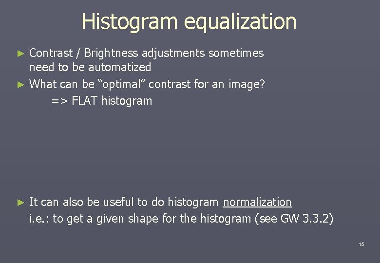
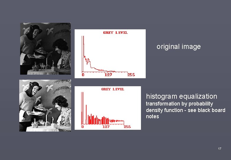
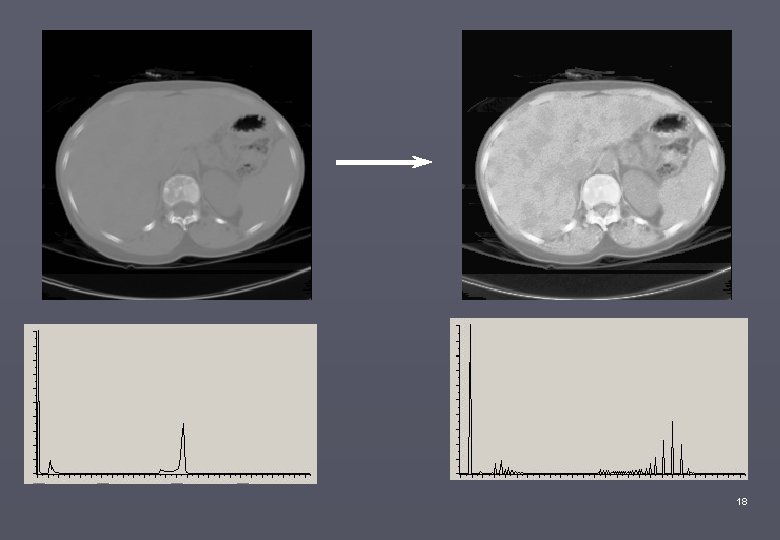
Histogram equalization Contrast / Brightness adjustments sometimes need to be automatized ► What can be “optimal” contrast for an image? => FLAT histogram ► ► It can also be useful to do histogram normalization i. e. : to get a given shape for the histogram (see GW 3. 3. 2) 15

Histogram Equalization, example quantization interval [0 7], image size 256 x 256 rk 0/7=0 1/7=0. 14 2/7=0. 29 3/7=0. 43 4/7=0. 57 5/7=0. 71 6/7=0. 86 7/7=1 nk 24979 21636 10865 3122 1411 656 2583 284 pr(rk) 0. 38 0. 33 0. 17 0. 05 0. 02 0. 01 0. 04 0. 00 sk 0. 38 0. 71 0. 88 0. 93 0. 95 0. 96 1. 00 output 3 5 6 6 7 7 16

original image histogram equalization transformation by probability density function - see black board notes 17

18

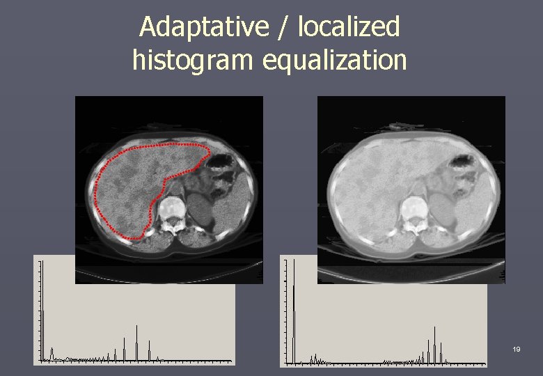
Adaptative / localized histogram equalization 19

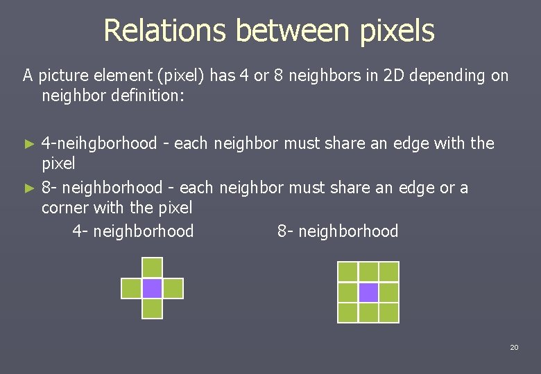
Relations between pixels A picture element (pixel) has 4 or 8 neighbors in 2 D depending on neighbor definition: 4 -neihgborhood - each neighbor must share an edge with the pixel ► 8 - neighborhood - each neighbor must share an edge or a corner with the pixel 4 - neighborhood 8 - neighborhood ► 20

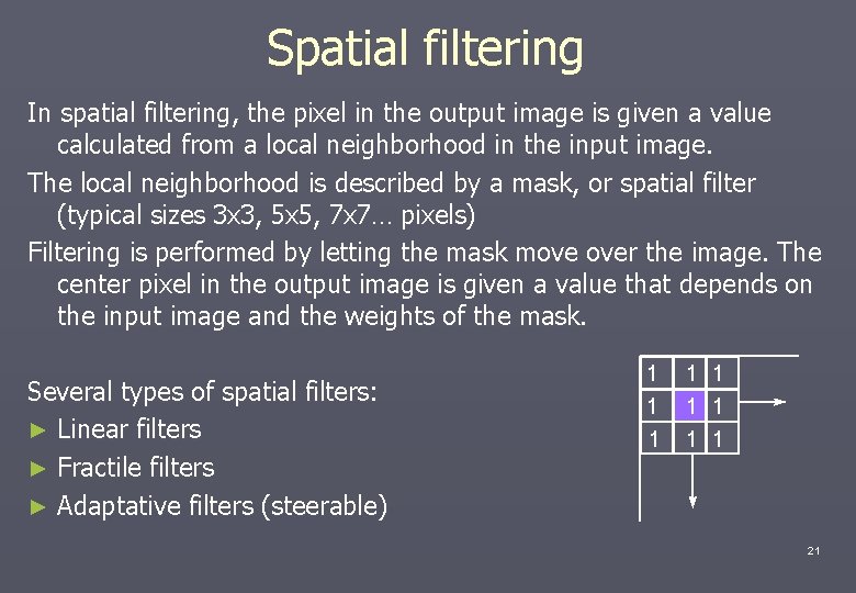
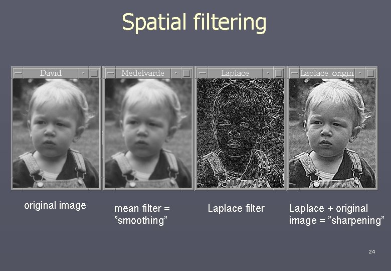
Spatial filtering In spatial filtering, the pixel in the output image is given a value calculated from a local neighborhood in the input image. The local neighborhood is described by a mask, or spatial filter (typical sizes 3 x 3, 5 x 5, 7 x 7… pixels) Filtering is performed by letting the mask move over the image. The center pixel in the output image is given a value that depends on the input image and the weights of the mask. Several types of spatial filters: ► Linear filters ► Fractile filters ► Adaptative filters (steerable) 1 1 1 1 1 21

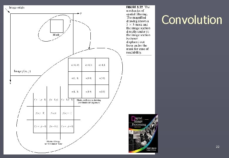
Convolution 22

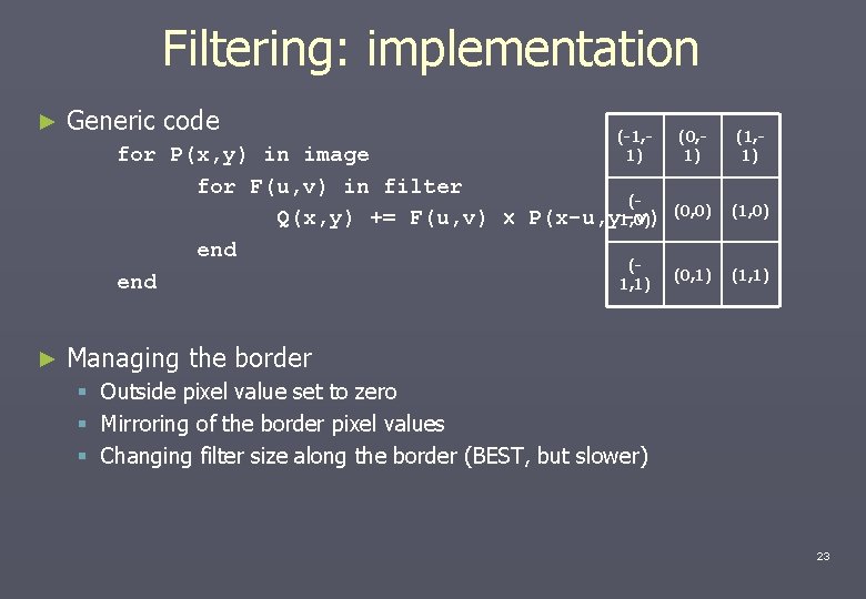
Filtering: implementation ► Generic code (-1, 1) for P(x, y) in image for F(u, v) in filter (Q(x, y) += F(u, v) P(x-u, y-v) 1, 0) end (end 1, 1) ► (0, 1) (1, 1) (0, 0) (1, 0) (0, 1) (1, 1) Managing the border § Outside pixel value set to zero § Mirroring of the border pixel values § Changing filter size along the border (BEST, but slower) 23

Spatial filtering original image mean filter = ”smoothing” Laplace filter Laplace + original image = ”sharpening” 24

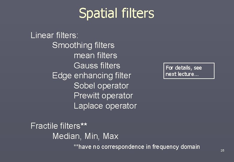
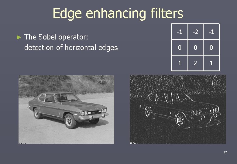
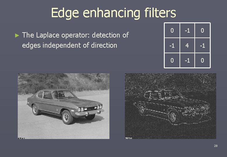
Spatial filters Linear filters: Smoothing filters mean filters Gauss filters Edge enhancing filter Sobel operator Prewitt operator Laplace operator For details, see next lecture… Fractile filters** Median, Min, Max **have no correspondence in frequency domain 25

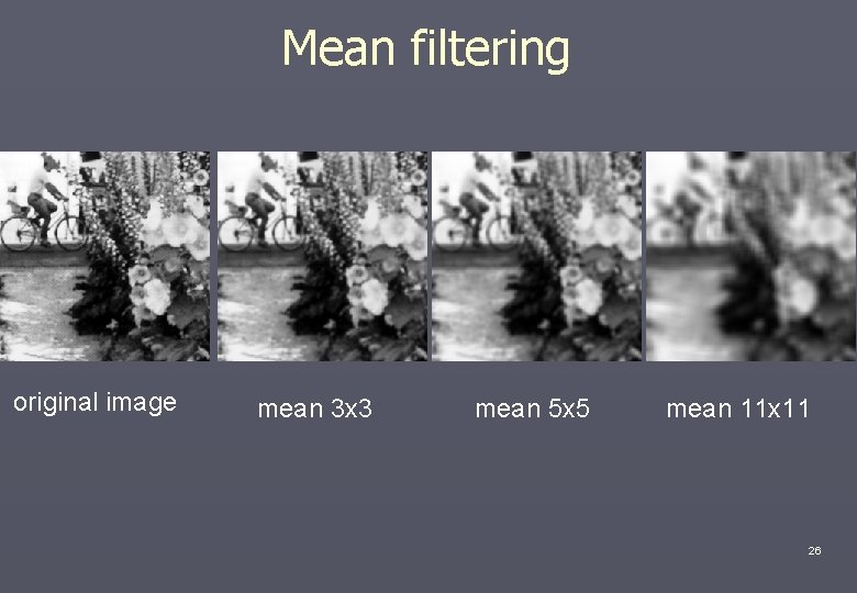
Mean filtering original image mean 3 x 3 mean 5 x 5 mean 11 x 11 26

Edge enhancing filters ► The Sobel operator: detection of horizontal edges -1 -2 -1 0 0 0 1 27

Edge enhancing filters ► The Laplace operator: detection of edges independent of direction 0 -1 4 -1 0 28