CS 584 Iterative Methods Gaussian elimination is considered

CS 584

Iterative Methods Gaussian elimination is considered to be a direct method to solve a system. n An indirect method produces a sequence of values that converges to the solution of the system. n Computation is halted in an indirect algorithm when a specified accuracy is reached. n

Why Iterative Methods? n Sometimes we don't need to be exact. – Input has inaccuracy, etc. – Only requires a few iterations If the system is sparse, the matrix can be stored in a different format. n Iterative methods are usually stable. n – Errors are dampened

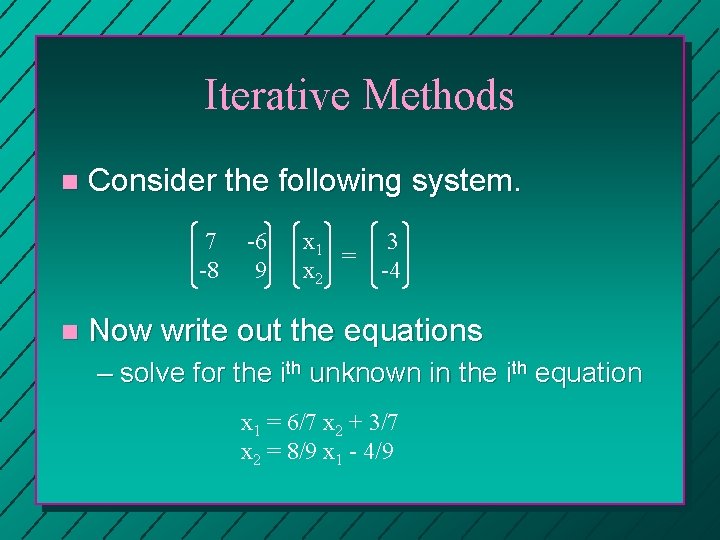
Iterative Methods n Consider the following system. 7 -8 n -6 9 x 1 = x 2 3 -4 Now write out the equations – solve for the ith unknown in the ith equation x 1 = 6/7 x 2 + 3/7 x 2 = 8/9 x 1 - 4/9

Iterative Methods n Come up with an initial guess for each xi n Hopefully, the equations will produce better values and which can be used to calculate better values, etc. and will converge to the answer.

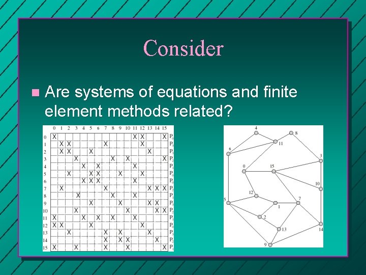
Consider n Are systems of equations and finite element methods related?

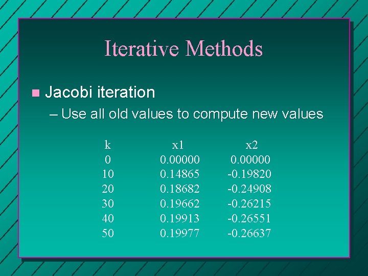
Iterative Methods n Jacobi iteration – Use all old values to compute new values k 0 10 20 30 40 50 x 1 0. 00000 0. 14865 0. 18682 0. 19662 0. 19913 0. 19977 x 2 0. 00000 -0. 19820 -0. 24908 -0. 26215 -0. 26551 -0. 26637

Jacobi Iteration n The ith equation has the form n -1 å A[i, j]x[ j ] = b[i] j =0 n Which can be rewritten as: ö 1 æç x[i ] = b[i ] - å A[i, j ]x[ j ]÷÷ ç A[i, i ] è j ¹i ø

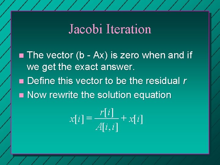
Jacobi Iteration The vector (b - Ax) is zero when and if we get the exact answer. n Define this vector to be the residual r n Now rewrite the solution equation n r[i ] + x[i ] = A[i, i ]

void Jacobi(float A[][], float b[], float x[], float epsilon) { int k = 0; float x 1[]; float r 0 norm; // Randomly select an initial x vector r = b - Ax; // This involves matrix-vector mult etc. r 0 norm = ||r||2; // This is basically the magnitude while (||r||2 > epsilon * r 0 norm) { for (j = 0; j < n; j++) x 1[j] = r[j] / A[j, j] + x[j]; r = b - Ax; } x = x 1; }

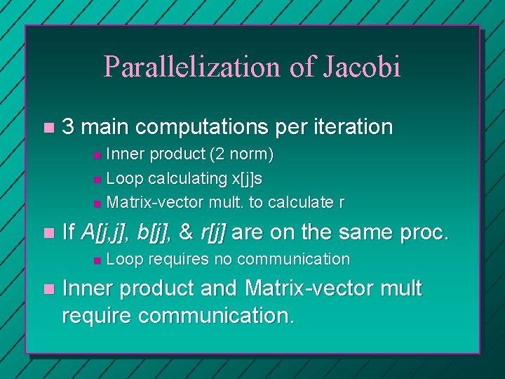
Parallelization of Jacobi n 3 main computations per iteration Inner product (2 norm) n Loop calculating x[j]s n Matrix-vector mult. to calculate r n n If A[j, j], b[j], & r[j] are on the same proc. n n Loop requires no communication Inner product and Matrix-vector mult require communication.

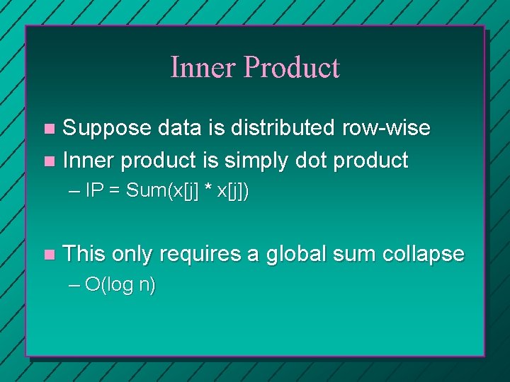
Inner Product Suppose data is distributed row-wise n Inner product is simply dot product n – IP = Sum(x[j] * x[j]) n This only requires a global sum collapse – O(log n)

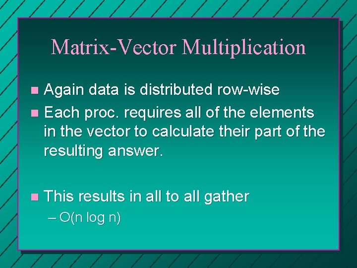
Matrix-Vector Multiplication Again data is distributed row-wise n Each proc. requires all of the elements in the vector to calculate their part of the resulting answer. n n This results in all to all gather – O(n log n)

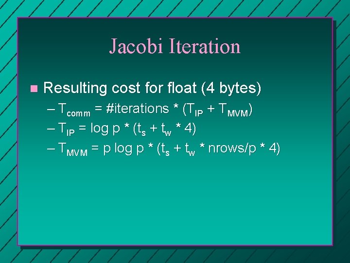
Jacobi Iteration n Resulting cost for float (4 bytes) – Tcomm = #iterations * (TIP + TMVM) – TIP = log p * (ts + tw * 4) – TMVM = p log p * (ts + tw * nrows/p * 4)

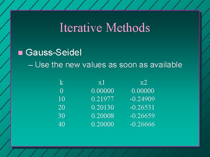
Iterative Methods n Gauss-Seidel – Use the new values as soon as available k 0 10 20 30 40 x 1 0. 00000 0. 21977 0. 20130 0. 20008 0. 20000 x 2 0. 00000 -0. 24909 -0. 26531 -0. 26659 -0. 26666

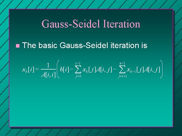
Gauss-Seidel Iteration n The basic Gauss-Seidel iteration is i -1 n -1 ö 1 æç ÷ xk [i ] = b [ i ] x [ j ] A [ i , j ] å å 1 k k ÷ A[i, i ] çè j =0 j = i +1 ø

Gauss-Seidel Iteration Rule: Always use the newest values of the previously computed variables. n Problem: Sequential? n Gauss-Seidel is indeed sequential if the matrix is dense. n Parallelism is a function of the sparsity and ordering of the equation matrix. n

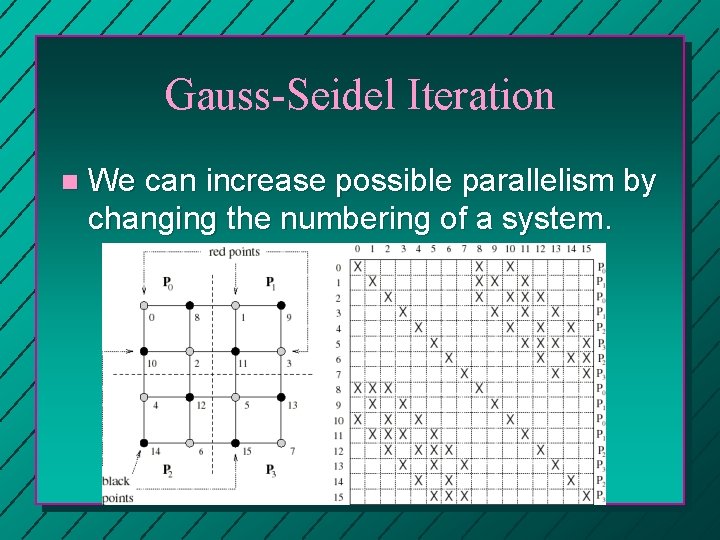
Gauss-Seidel Iteration n We can increase possible parallelism by changing the numbering of a system.

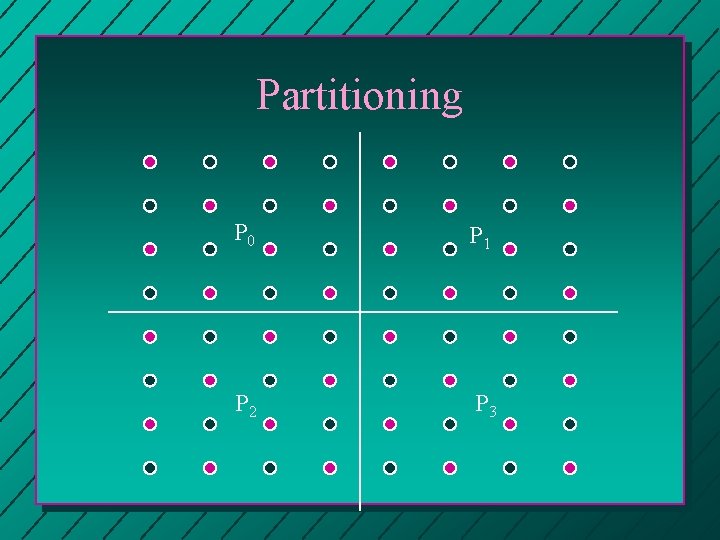
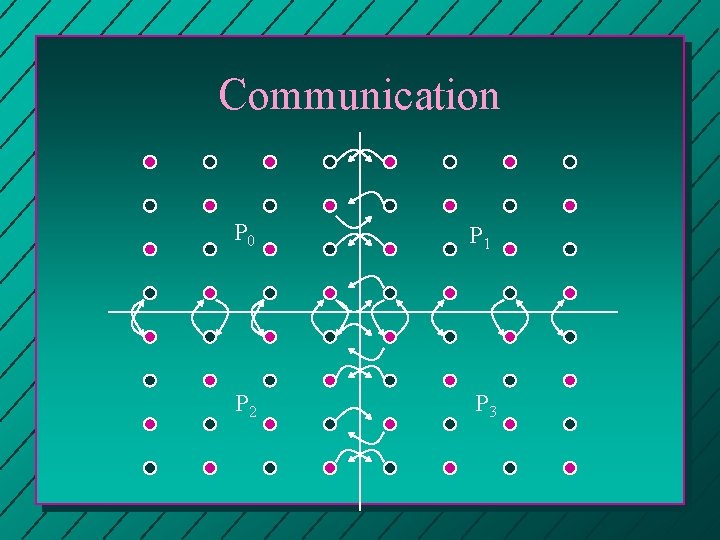
Parallelizing Red-Black GSI n Partitioning? Block checkerboard. n Communication? 2 phases per iteration. 1 - compute red cells using values from black cells 2 - compute black cells using values from red cells Communication is required for each phase.

Partitioning P 0 P 1 P 2 P 3

Communication P 0 P 1 P 2 P 3

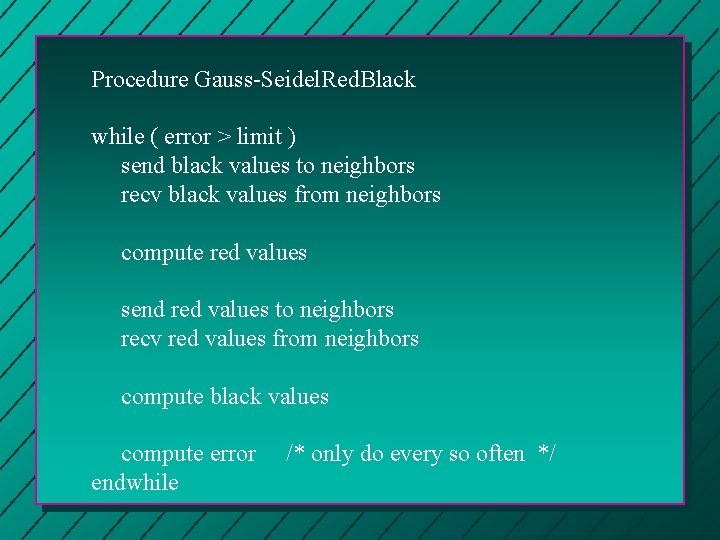
Procedure Gauss-Seidel. Red. Black while ( error > limit ) send black values to neighbors recv black values from neighbors compute red values send red values to neighbors recv red values from neighbors compute black values compute error endwhile /* only do every so often */

Extending Red-Black Coloring Goal: Produce a graph coloring scheme such that no node has a neighbor of the same color. n Finite element methods produce graphs with only 4 neighbors. n – Two colors suffice n What about more complex graphs?

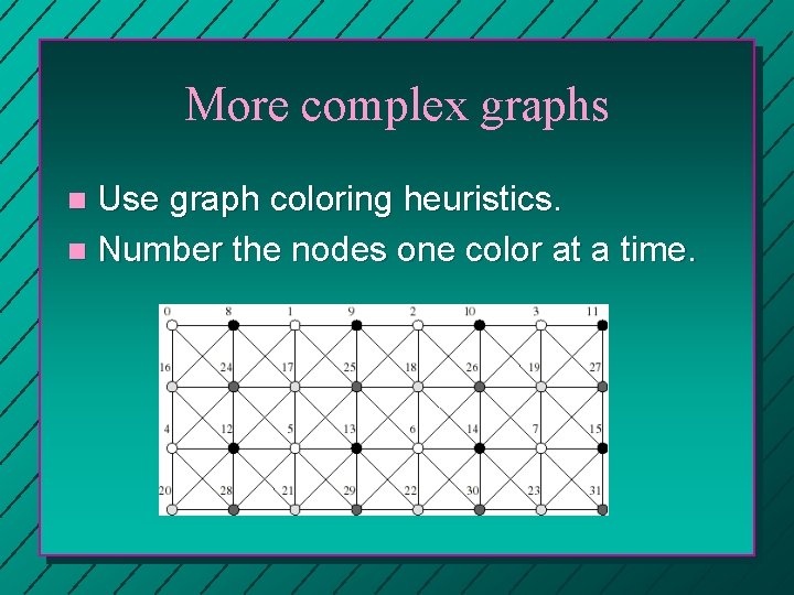
More complex graphs Use graph coloring heuristics. n Number the nodes one color at a time. n

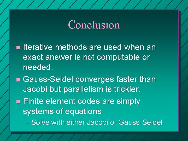
Conclusion Iterative methods are used when an exact answer is not computable or needed. n Gauss-Seidel converges faster than Jacobi but parallelism is trickier. n Finite element codes are simply systems of equations n – Solve with either Jacobi or Gauss-Seidel