Chapter 4 Money and Inflation MACROECONOMICS Seventh Edition

Chapter 4: Money and Inflation* MACROECONOMICS Seventh Edition N. Gregory Mankiw *Slides based on Ron Cronovich's slides, adjusted for course in Macroeconomics Chapter 4: Money and Inflation 1/67

4. 2) The Quantity Theory of Money Provides the leading explanation of how money affects the economy in the long run. A simple theory linking the inflation rate to the growth rate of the money supply. Begins with the concept of velocity… Chapter 4: Money and Inflation 12/67

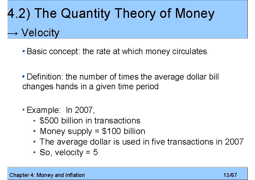
4. 2) The Quantity Theory of Money → Velocity Basic concept: the rate at which money circulates Definition: the number of times the average dollar bill changes hands in a given time period Example: In 2007, $500 billion in transactions Money supply = $100 billion The average dollar is used in five transactions in 2007 So, velocity = 5 Chapter 4: Money and Inflation 13/67

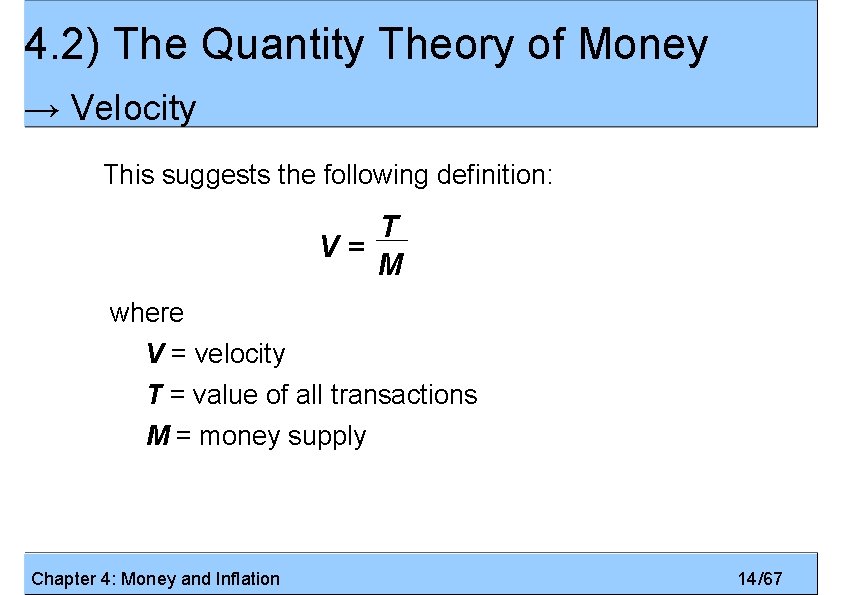
4. 2) The Quantity Theory of Money → Velocity This suggests the following definition: T V= M where V = velocity T = value of all transactions M = money supply Chapter 4: Money and Inflation 14/67

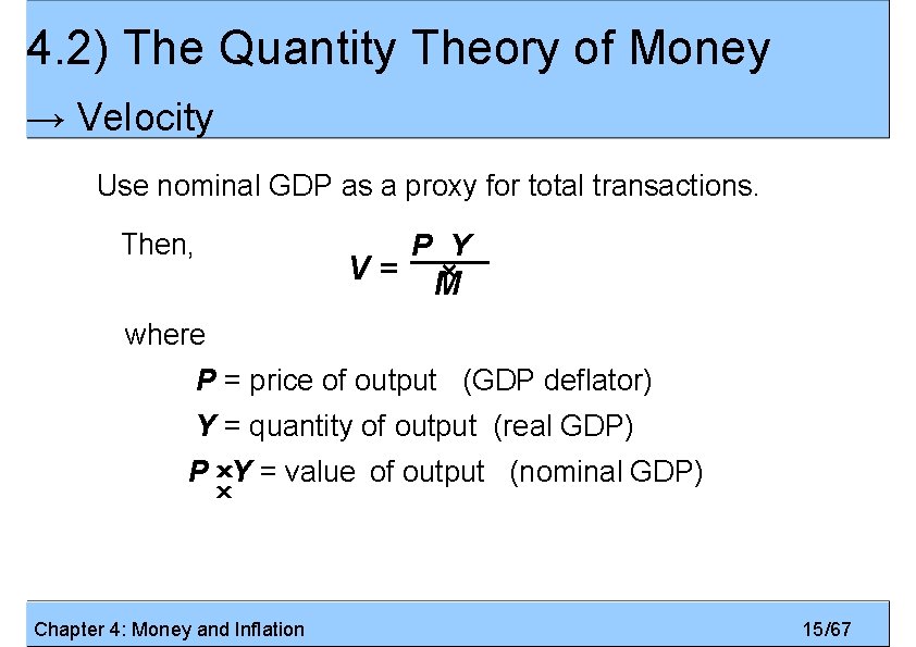
4. 2) The Quantity Theory of Money → Velocity Use nominal GDP as a proxy for total transactions. Then, V= P Y × M where P = price of output (GDP deflator) Y = quantity of output (real GDP) P ×Y × = value of output (nominal GDP) × Chapter 4: Money and Inflation 15/67

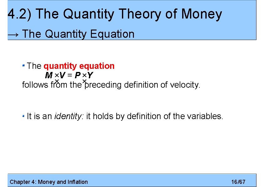
4. 2) The Quantity Theory of Money → The Quantity Equation The quantity equation M ×V = P ×Y × the×preceding definition of velocity. follows from It is an identity: it holds by definition of the variables. Chapter 4: Money and Inflation 16/67

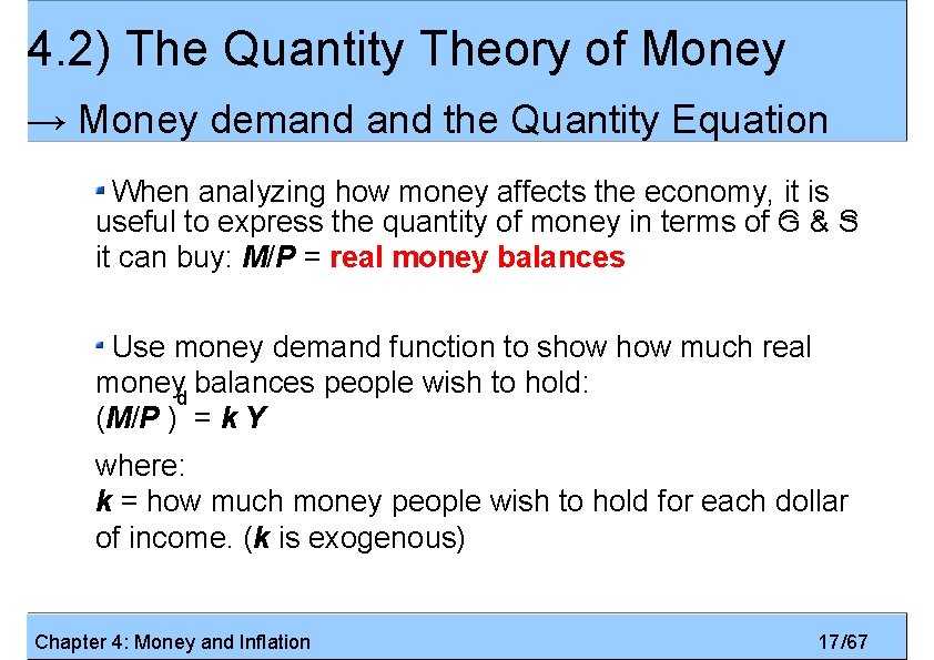
4. 2) The Quantity Theory of Money → Money demand the Quantity Equation When analyzing how money affects the economy, it is useful to to express the quantity of of money in in terms of of G G& &S S it can buy: M/P = real money balances Use money demand function to show much real moneyd balances people wish to hold: (M/P ) = k Y where: k = how much money people wish to hold for each dollar of income. (k is exogenous) Chapter 4: Money and Inflation 17/67

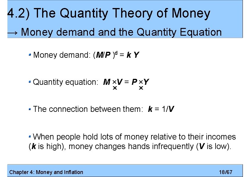
4. 2) The Quantity Theory of Money → Money demand the Quantity Equation Money demand: (M/P )d = k Y Quantity equation: M ×V = P ×Y × × The connection between them: k = 1/V When people hold lots of money relative to their incomes (k is high), money changes hands infrequently (V is low). Chapter 4: Money and Inflation 18/67

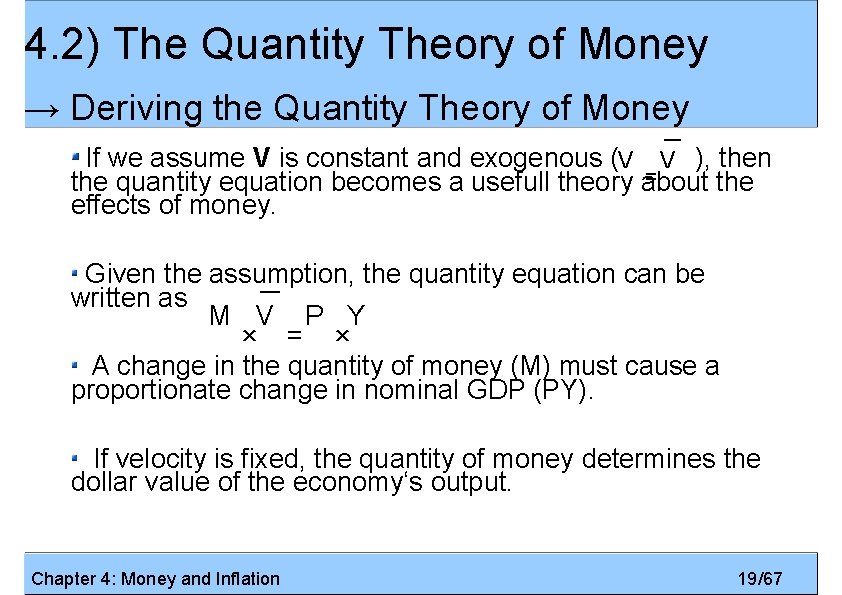
4. 2) The Quantity Theory of Money → Deriving the Quantity Theory of Money If we assume V is constant and exogenous (V V ), then = the quantity equation becomes a usefull theory about the effects of money. Given the assumption, the quantity equation can be written as M V P Y × = × A change in the quantity of money (M) must cause a proportionate change in nominal GDP (PY). If velocity is fixed, the quantity of money determines the dollar value of the economy‘s output. Chapter 4: Money and Inflation 19/67

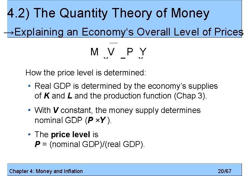
4. 2) The Quantity Theory of Money →Explaining an Economy‘s Overall Level of Prices M V P Y × = × How the price level is determined: Real GDP is determined by the economy’s supplies of K and L and the production function (Chap 3). With V constant, the money supply determines nominal GDP (P ×Y ). The price level is P = (nominal GDP)/(real GDP). Chapter 4: Money and Inflation 20/67

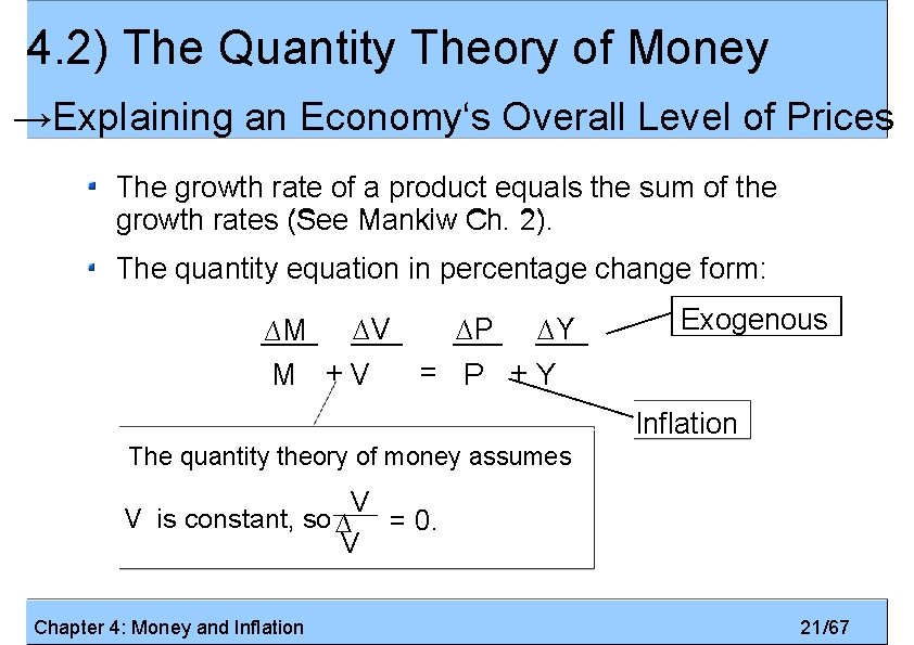
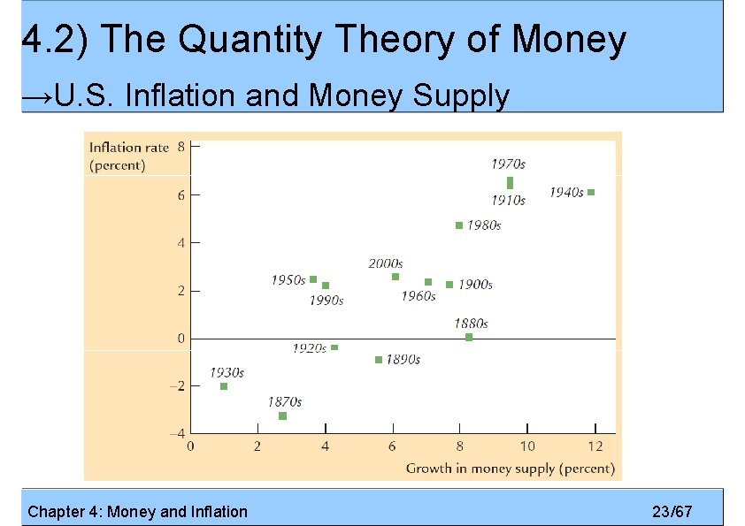
4. 2) The Quantity Theory of Money →Explaining an Economy‘s Overall Level of Prices The growth rate of a product equals the sum of the growth rates (See Mankiw Ch. 2). The quantity equation in percentage change form: ∆P ∆Y ∆M ∆V = P +Y M +V Exogenous Inflation The quantity theory of money assumes V V is constant, so ∆ = 0. V Chapter 4: Money and Inflation 21/67

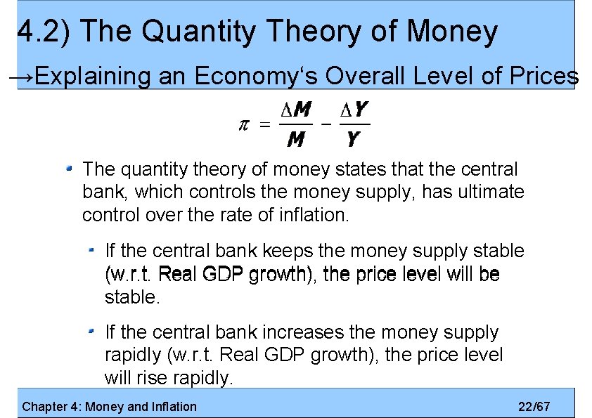
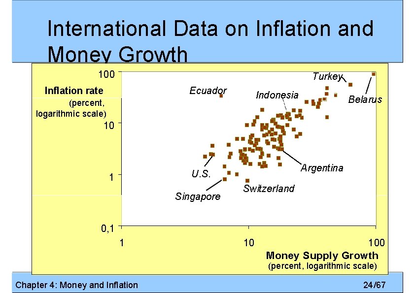
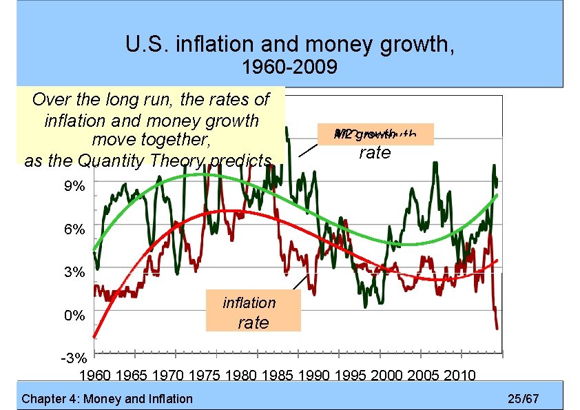
4. 2) The Quantity Theory of Money →Explaining an Economy‘s Overall Level of Prices The quantity theory of money states that the central bank, which controls the money supply, has ultimate control over the rate of inflation. If the central bank keeps the money supply stable (w. r. t. Real GDP growth), the price level will be stable. If the central bank increases the money supply rapidly (w. r. t. Real GDP growth), the price level will rise rapidly. Chapter 4: Money and Inflation 22/67

4. 2) The Quantity Theory of Money →U. S. Inflation and Money Supply Chapter 4: Money and Inflation 23/67

International Data on Inflation and Money Growth 100 Turkey Ecuador Inflation rate Indonesia (percent, logarithmic scale) Belarus 10 Argentina U. S. 1 Singapore Switzerland 0, 1 1 10 100 Money Supply Growth (percent, logarithmic scale) Chapter 4: Money and Inflation 24/67

U. S. inflation and money growth, 1960 -2009 15% Over the long run, the rates of inflation and money growth 12% move together, as the Quantity Theory predicts. M 2 growth rate 9% 6% 3% 0% inflation rate -3% 1960 1965 1970 1975 1980 1985 1990 1995 2000 2005 2010 Chapter 4: Money and Inflation 25/67