ZPL A Parallel Programming Language ZPL is an

ZPL, A Parallel Programming Language ZPL is an implicitly parallel array programming language based on the CTA machine model. Though designed for scientific computation, ZPL illustrates fundamental ideas in parallel computing essential to all application areas. 1 Copyright, Lawrence Snyder, 1999

Practical Considerations • The purpose of learning ZPL is to illustrate the fundamental point from the first lecture that a parallel machine model enables one to write programs independent of target machine, yet still have sufficient understanding of their performance to estimate how they will run • Find documentation on the ZPL home page: www. cs. washington. edu/research/zpl/docs/descriptions/guide. html • ZPL has been installed on orcas/sanjuan 2 Copyright, Lawrence Snyder, 1999

Homework Assignment • This lecture provides sufficient instruction to write many ZPL programs • Two straightforward computations are • Game of Life • All Pairs Shortest Path, based on Warshall’s Algorithm • These problems are further specified on the class web page 3 Copyright, Lawrence Snyder, 1999

ZPL Overview • ZPL’s main data structure is a dense array • Computation is expressed as operations on whole arrays, ie A+B adds arrays elementwise • Parallelism is implicit, i. e. inferred by the compiler from the array expressions • ZPL is compiled, not interactive like MATLAB • ZPL compiles to ANSI C which is compiled with machine specific libraries to the target parallel computer 4 Copyright, Lawrence Snyder, 1999

ZPL Factoids • Development Milestones • ZPL design & implementation began in 3/93 • Portability & performance demonstrated 7/94 • Compiler and run-time system released 7/97 • Claims • Portable to any (MIMD) parallel computer • Performance comparable to C with user specified communication • Generally out performs High Performance Fortran • Convenient and intuitive • ZPL is a proper subset of Advanced ZPL 5 Copyright, Lawrence Snyder, 1999

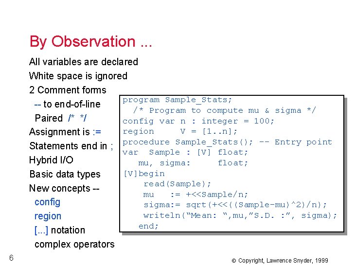
By Observation. . . All variables are declared White space is ignored 2 Comment forms program Sample_Stats; -- to end-of-line /* Program to compute mu & sigma */ Paired /* */ config var n : integer = 100; region V = [1. . n]; Assignment is : = procedure Sample_Stats(); -- Entry point Statements end in ; var Sample : [V] float; Hybrid I/O mu, sigma: float; [V]begin Basic data types read(Sample); New concepts -mu : = +<<Sample/n; config sigma: = sqrt(+<<((Sample-mu)^2)/n); writeln(“Mean: “, mu, ”S. D. : ”, sigma); region end; [. . . ] notation complex operators 6 Copyright, Lawrence Snyder, 1999

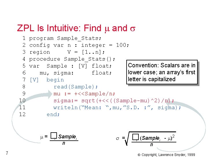
ZPL Is Intuitive: Find and 1 2 3 4 5 6 7 8 9 10 11 12 program Sample_Stats; config var n : integer = 100; region V = [1. . n]; procedure Sample_Stats(); Convention: Scalars are in var Sample : [V] float; lower case; an array’s first mu, sigma: float; letter is capitalized [V] begin read(Sample); mu : = +<<Sample/n; sigma: = sqrt(+<<((Sample-mu)^2)/n); writeln(“Mean: “, mu, ”S. D. : ”, sigma); end; = 7 �Sample i n i = �(Sample i n i - )2 Copyright, Lawrence Snyder, 1999

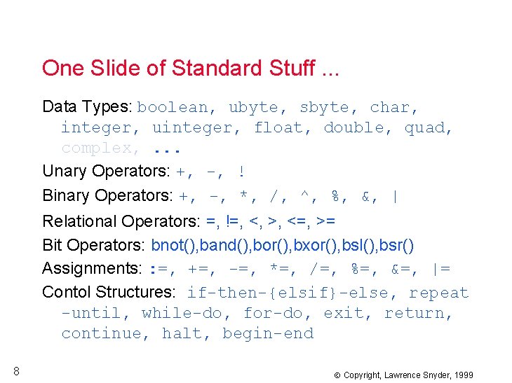
One Slide of Standard Stuff. . . Data Types: boolean, ubyte, sbyte, char, integer, uinteger, float, double, quad, complex, . . . Unary Operators: +, -, ! Binary Operators: +, -, *, /, ^, %, &, | Relational Operators: =, !=, <, >, <=, >= Bit Operators: bnot(), band(), bor(), bxor(), bsl(), bsr() Assignments: : =, +=, -=, *=, /=, %=, &=, |= Contol Structures: if-then-{elsif}-else, repeat -until, while-do, for-do, exit, return, continue, halt, begin-end 8 Copyright, Lawrence Snyder, 1999

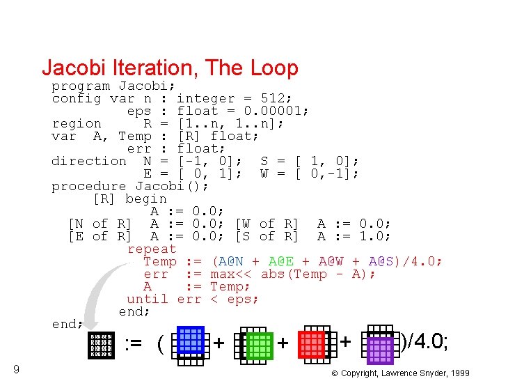
Jacobi Iteration, The Loop program Jacobi; config var n : integer = 512; eps : float = 0. 00001; region R = [1. . n, 1. . n]; var A, Temp : [R] float; err : float; direction N = [-1, 0]; S = [ 1, 0]; E = [ 0, 1]; W = [ 0, -1]; procedure Jacobi(); [R] begin A : = 0. 0; [N of R] A : = 0. 0; [W of R] A : = 0. 0; [E of R] A : = 0. 0; [S of R] A : = 1. 0; repeat Temp : = (A@N + A@E + A@W + A@S)/4. 0; err : = max<< abs(Temp - A); A : = Temp; until err < eps; end; : = ( 9 + + + )/4. 0; Copyright, Lawrence Snyder, 1999

Jacobi Iteration, The Region program Jacobi; config var n : integer = 512; eps : float = 0. 00001; region R = [1. . n, 1. . n]; var A, Temp : [R] float; err : float; direction N = [-1, 0]; S = [ 1, 0]; E = [ 0, 1]; W = [ 0, -1]; procedure Jacobi(); [R] begin A : = 0. 0; [N of R] A : = 0. 0; [W of R] A : = 0. 0; [E of R] A : = 0. 0; [S of R] A : = 1. 0; repeat Temp : = (A@N + A@E + A@W + A@S)/4. 0; err : = max<< abs(Temp - A); A : = Temp; until err < eps; end; 10 Copyright, Lawrence Snyder, 1999

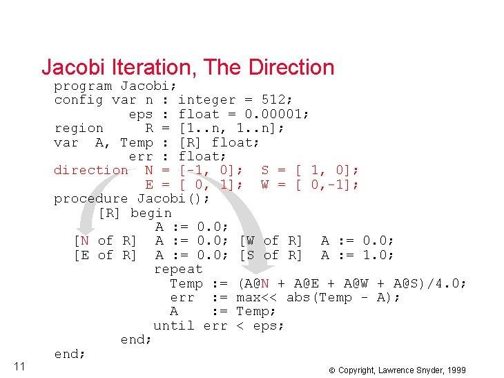
Jacobi Iteration, The Direction 11 program Jacobi; config var n : integer = 512; eps : float = 0. 00001; region R = [1. . n, 1. . n]; var A, Temp : [R] float; err : float; direction N = [-1, 0]; S = [ 1, 0]; E = [ 0, 1]; W = [ 0, -1]; procedure Jacobi(); [R] begin A : = 0. 0; [N of R] A : = 0. 0; [W of R] A : = 0. 0; [E of R] A : = 0. 0; [S of R] A : = 1. 0; repeat Temp : = (A@N + A@E + A@W + A@S)/4. 0; err : = max<< abs(Temp - A); A : = Temp; until err < eps; end; Copyright, Lawrence Snyder, 1999

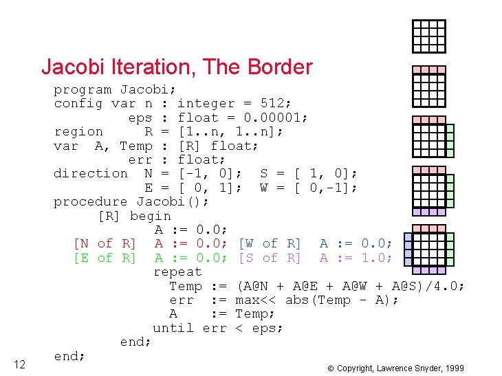
Jacobi Iteration, The Border 12 program Jacobi; config var n : integer = 512; eps : float = 0. 00001; region R = [1. . n, 1. . n]; var A, Temp : [R] float; err : float; direction N = [-1, 0]; S = [ 1, 0]; E = [ 0, 1]; W = [ 0, -1]; procedure Jacobi(); [R] begin A : = 0. 0; [N of R] A : = 0. 0; [W of R] A : = 0. 0; [E of R] A : = 0. 0; [S of R] A : = 1. 0; repeat Temp : = (A@N + A@E + A@W + A@S)/4. 0; err : = max<< abs(Temp - A); A : = Temp; until err < eps; end; Copyright, Lawrence Snyder, 1999

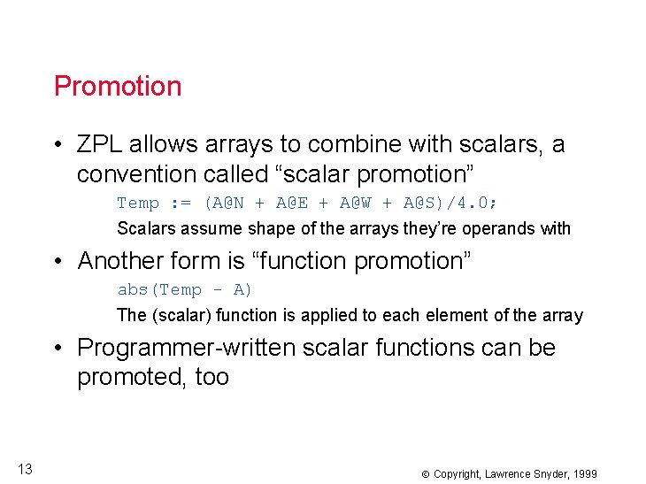
Promotion • ZPL allows arrays to combine with scalars, a convention called “scalar promotion” Temp : = (A@N + A@E + A@W + A@S)/4. 0; Scalars assume shape of the arrays they’re operands with • Another form is “function promotion” abs(Temp - A) The (scalar) function is applied to each element of the array • Programmer-written scalar functions can be promoted, too 13 Copyright, Lawrence Snyder, 1999

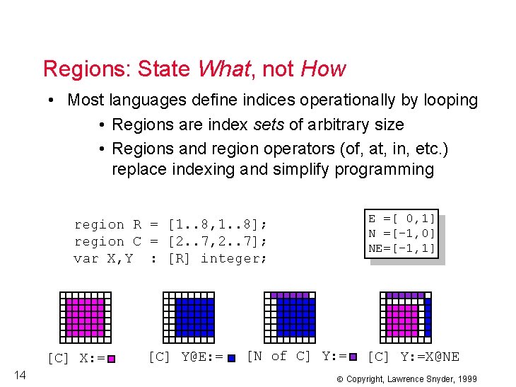
Regions: State What, not How • Most languages define indices operationally by looping • Regions are index sets of arbitrary size • Regions and region operators (of, at, in, etc. ) replace indexing and simplify programming E =[ 0, 1] N =[-1, 0] NE=[-1, 1] region R = [1. . 8, 1. . 8]; region C = [2. . 7, 2. . 7]; var X, Y : [R] integer; [C] X: = 14 [C] Y@E: = [N of C] Y: = [C] Y: =X@NE Copyright, Lawrence Snyder, 1999

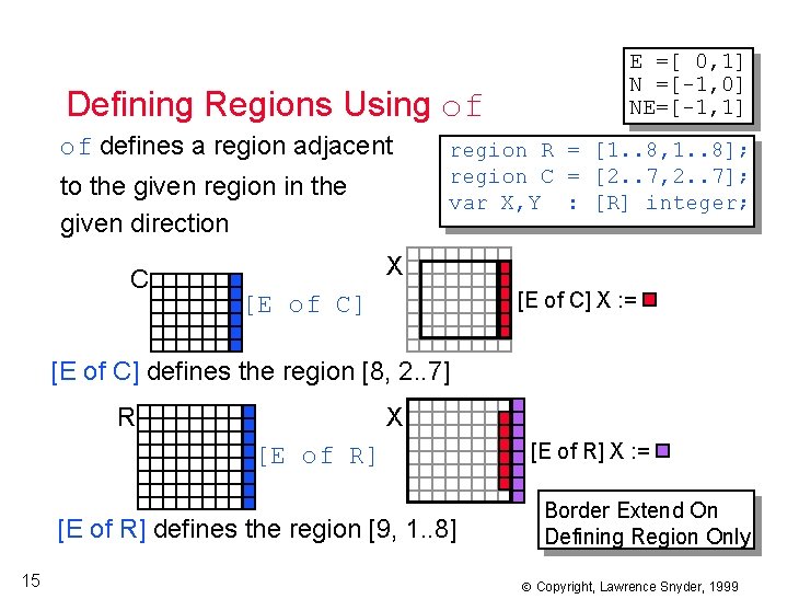
Defining Regions Using of of defines a region adjacent to the given region in the given direction C E =[ 0, 1] N =[-1, 0] NE=[-1, 1] region R = [1. . 8, 1. . 8]; region C = [2. . 7, 2. . 7]; var X, Y : [R] integer; X [E of C] X : = [E of C] defines the region [8, 2. . 7] R X [E of R] defines the region [9, 1. . 8] 15 [E of R] X : = Border Extend On Defining Region Only Copyright, Lawrence Snyder, 1999

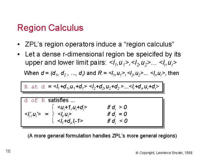
Region Calculus • ZPL’s region operators induce a “region calculus” • Let a dense r-dimensional region be speicifed by its upper and lower limit pairs: <l 1, u 1>, <l 2, u 2>. . . <lr, ur> When d = (d 1, d 2 , . . . , dr) and R = <l 1, u 1>, <l 2, u 2>. . . <lr, ur>, then R at d = <l 1+d 1, u 1+d 1> <l 2+d 2, u 2+d 2 >. . . <lr+dr, ur+dr> d of R satisfies. . . <ui+1, ui+di> <li’, ui’> = <li, ui> <l 1+di, li-1> if di > 0 if di = 0 if di < 0 (A more general formulation handles ZPL’s more general regions) 16 Copyright, Lawrence Snyder, 1999

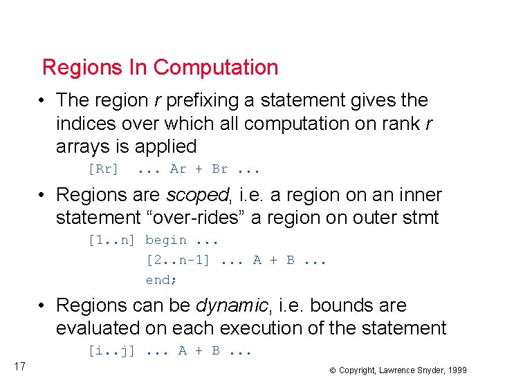
Regions In Computation • The region r prefixing a statement gives the indices over which all computation on rank r arrays is applied [Rr] . . . Ar + Br. . . • Regions are scoped, i. e. a region on an inner statement “over-rides” a region on outer stmt [1. . n] begin. . . [2. . n-1]. . . A + B. . . end; • Regions can be dynamic, i. e. bounds are evaluated on each execution of the statement [i. . j]. . . A + B. . . 17 Copyright, Lawrence Snyder, 1999

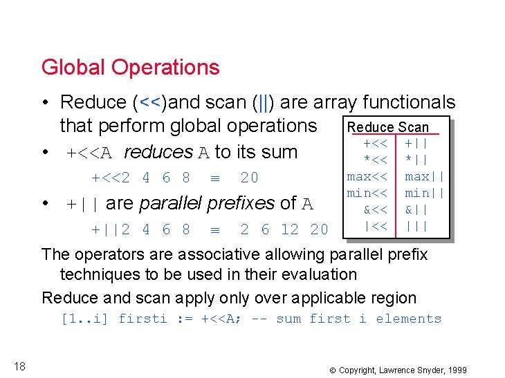
Global Operations • Reduce (<<)and scan (||) are array functionals that perform global operations Reduce Scan +<< +|| • +<<A reduces A to its sum *<< *|| +<<2 4 6 8 20 • +|| are parallel prefixes of A +||2 4 6 8 2 6 12 20 max<< min<< &<< |<< max|| min|| &|| ||| The operators are associative allowing parallel prefix techniques to be used in their evaluation Reduce and scan apply only over applicable region [1. . i] firsti : = +<<A; -- sum first i elements 18 Copyright, Lawrence Snyder, 1999

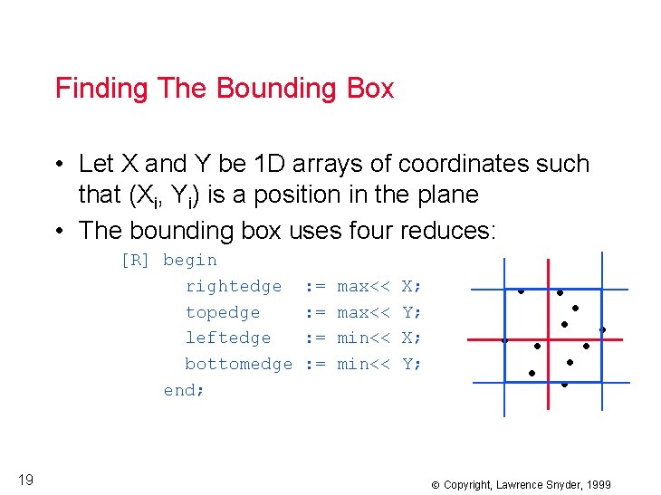
Finding The Bounding Box • Let X and Y be 1 D arrays of coordinates such that (Xi, Yi) is a position in the plane • The bounding box uses four reduces: [R] begin rightedge topedge leftedge bottomedge end; 19 : = : = max<< min<< X; Y; • • • • Copyright, Lawrence Snyder, 1999

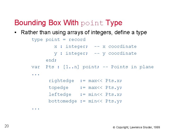
Bounding Box With point Type • Rather than using arrays of integers, define a type point = record x : integer; -- x coordinate y : integer; -- y coordinate end; var Pts : [1. . n] point; -- Points in plane. . . rightedge : = max<< Pts. x; topedge : = max<< Pts. y; leftedge : = min<< Pts. x; bottomedge : = min<< Pts. y; . . . 20 Copyright, Lawrence Snyder, 1999

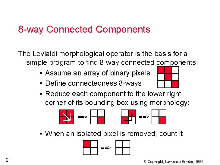
8 -way Connected Components The Levialdi morphological operator is the basis for a simple program to find 8 -way connected components • Assume an array of binary pixels • Define connectedness 8 -ways • Reduce each component to the lower right corner of its bounding box using morphology: ==> • When an isolated pixel is removed, count it ==> 21 Copyright, Lawrence Snyder, 1999

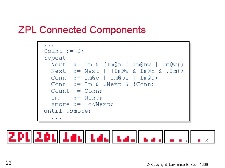
ZPL Connected Components. . . Count : = 0; repeat Next : = Im & (Im@n | Next : = Next | (Im@w Conn : = Im@e | Im@se Conn : = Im & !Next & Count += Conn; Im : = Next; smore : = |<<Next; until !smore; . . . 22 Im@nw | Im@w); & Im@n & !Im); | Im@s; !Conn; Copyright, Lawrence Snyder, 1999

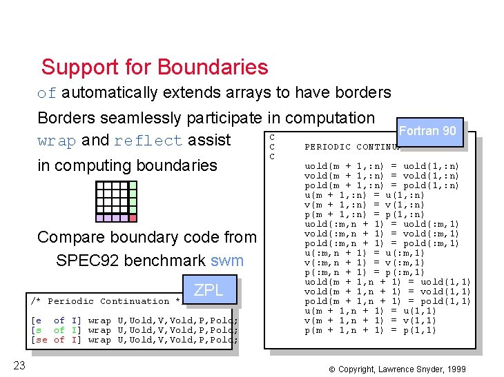
Support for Boundaries of automatically extends arrays to have borders Borders seamlessly participate in computation Fortran 90 C wrap and reflect assist C PERIODIC CONTINUATION in computing boundaries Compare boundary code from SPEC 92 benchmark swm /* Periodic Continuation */ ZPL [e of I] wrap U, Uold, V, Vold, P, Pold; [se of I] wrap U, Uold, V, Vold, P, Pold; 23 C uold(m + 1, : n) = uold(1, : n) vold(m + 1, : n) = vold(1, : n) pold(m + 1, : n) = pold(1, : n) u(m + 1, : n) = u(1, : n) v(m + 1, : n) = v(1, : n) p(m + 1, : n) = p(1, : n) uold(: m, n + 1) = uold(: m, 1) vold(: m, n + 1) = vold(: m, 1) pold(: m, n + 1) = pold(: m, 1) u(: m, n + 1) = u(: m, 1) v(: m, n + 1) = v(: m, 1) p(: m, n + 1) = p(: m, 1) uold(m + 1, n + 1) = uold(1, 1) vold(m + 1, n + 1) = vold(1, 1) pold(m + 1, n + 1) = pold(1, 1) u(m + 1, n + 1) = u(1, 1) v(m + 1, n + 1) = v(1, 1) p(m + 1, n + 1) = p(1, 1) Copyright, Lawrence Snyder, 1999

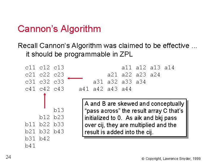
Cannon’s Algorithm Recall Cannon’s Algorithm was claimed to be effective. . . it should be programmable in ZPL c 11 c 21 c 31 c 41 c 12 c 22 c 32 c 42 c 13 c 23 c 33 c 43 b 12 b 23 b 11 b 22 b 33 b 21 b 32 b 43 b 31 b 42 b 41 24 a 11 a 12 a 13 a 14 a 21 a 22 a 23 a 24 a 31 a 32 a 33 a 34 a 41 a 42 a 43 a 44 A and B are skewed and conceptually “pass across” the result array C that’s initialized to 0. As aik and bkj pass over cij, they are multiplied and the result is added into the cij. Copyright, Lawrence Snyder, 1999

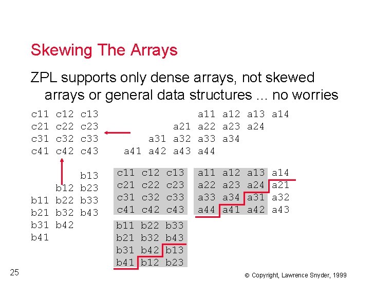
Skewing The Arrays ZPL supports only dense arrays, not skewed arrays or general data structures. . . no worries c 11 c 21 c 31 c 41 c 12 c 22 c 32 c 42 c 13 c 23 c 33 c 43 b 12 b 23 b 11 b 22 b 33 b 21 b 32 b 43 b 31 b 42 b 41 25 a 11 a 12 a 13 a 14 a 21 a 22 a 23 a 24 a 31 a 32 a 33 a 34 a 41 a 42 a 43 a 44 c 11 c 21 c 31 c 41 c 12 c 22 c 32 c 42 c 13 c 23 c 33 c 43 b 11 b 21 b 31 b 41 b 22 b 32 b 42 b 12 b 33 b 43 b 13 b 23 a 11 a 22 a 33 a 44 a 12 a 23 a 34 a 41 a 13 a 24 a 31 a 42 a 14 a 21 a 32 a 43 Copyright, Lawrence Snyder, 1999

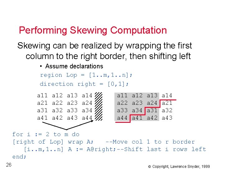
Performing Skewing Computation Skewing can be realized by wrapping the first column to the right border, then shifting left • Assume declarations region Lop = [1. . m, 1. . n]; direction right = [0, 1]; a 11 a 21 a 31 a 41 a 12 a 22 a 32 a 42 a 13 a 23 a 33 a 43 a 14 a 24 a 34 a 44 a 11 a 22 a 33 a 44 a 12 a 23 a 34 a 41 a 13 a 24 a 31 a 42 a 14 a 21 a 32 a 43 for i : = 2 to m do [right of Lop] wrap A; --Move col 1 to r border [i. . m, 1. . n] A : = A@right; --Shift last i rows left end; 26 Copyright, Lawrence Snyder, 1999

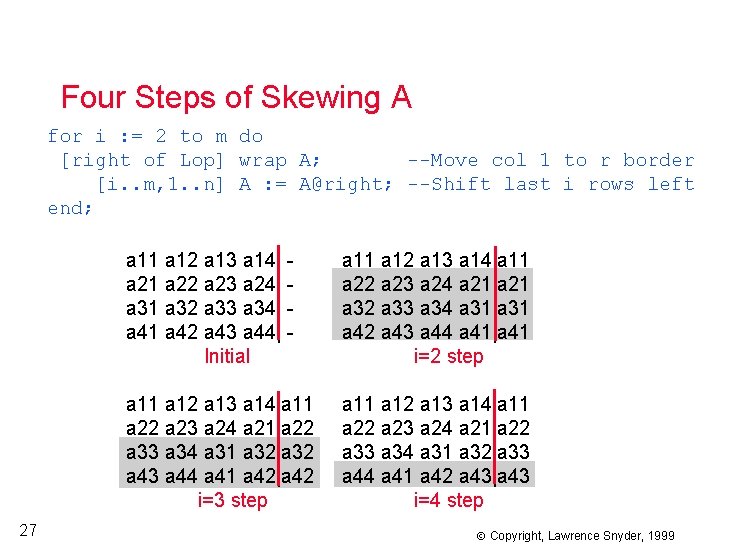
Four Steps of Skewing A for i : = 2 to m do [right of Lop] wrap A; --Move col 1 to r border [i. . m, 1. . n] A : = A@right; --Shift last i rows left end; 27 a 11 a 12 a 13 a 14| a 21 a 22 a 23 a 24| a 31 a 32 a 33 a 34| a 41 a 42 a 43 a 44| Initial a 11 a 12 a 13 a 14|a 11 a 22 a 23 a 24 a 21|a 21 a 32 a 33 a 34 a 31|a 31 a 42 a 43 a 44 a 41|a 41 i=2 step a 11 a 12 a 13 a 14|a 11 a 22 a 23 a 24 a 21|a 22 a 33 a 34 a 31 a 32|a 32 a 43 a 44 a 41 a 42|a 42 i=3 step a 11 a 12 a 13 a 14|a 11 a 22 a 23 a 24 a 21|a 22 a 33 a 34 a 31 a 32|a 33 a 44 a 41 a 42 a 43|a 43 i=4 step Copyright, Lawrence Snyder, 1999

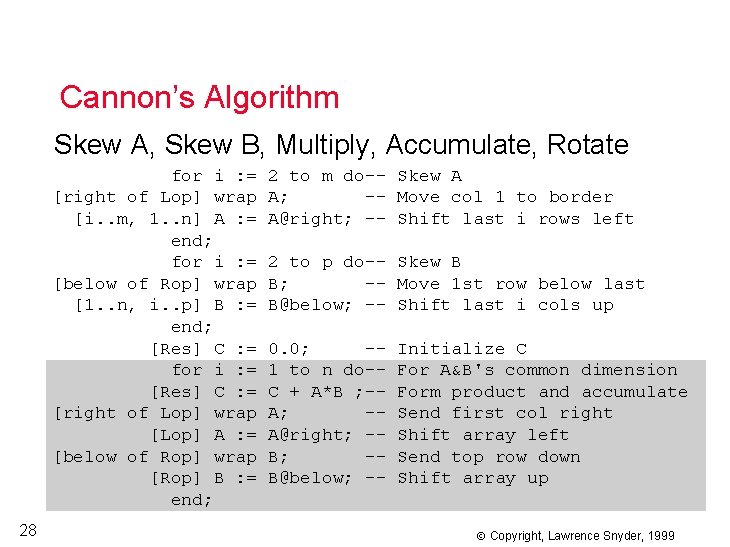
Cannon’s Algorithm Skew A, Skew B, Multiply, Accumulate, Rotate for i : = [right of Lop] wrap [i. . m, 1. . n] A : = end; for i : = [below of Rop] wrap [1. . n, i. . p] B : = end; [Res] C : = for i : = [Res] C : = [right of Lop] wrap [Lop] A : = [below of Rop] wrap [Rop] B : = end; 28 2 to m do-- Skew A A; -- Move col 1 to border A@right; -- Shift last i rows left 2 to p do-- Skew B B; -- Move 1 st row below last B@below; -- Shift last i cols up 0. 0; -1 to n do-C + A*B ; -A@right; -B@below; -- Initialize C For A&B's common dimension Form product and accumulate Send first col right Shift array left Send top row down Shift array up Copyright, Lawrence Snyder, 1999

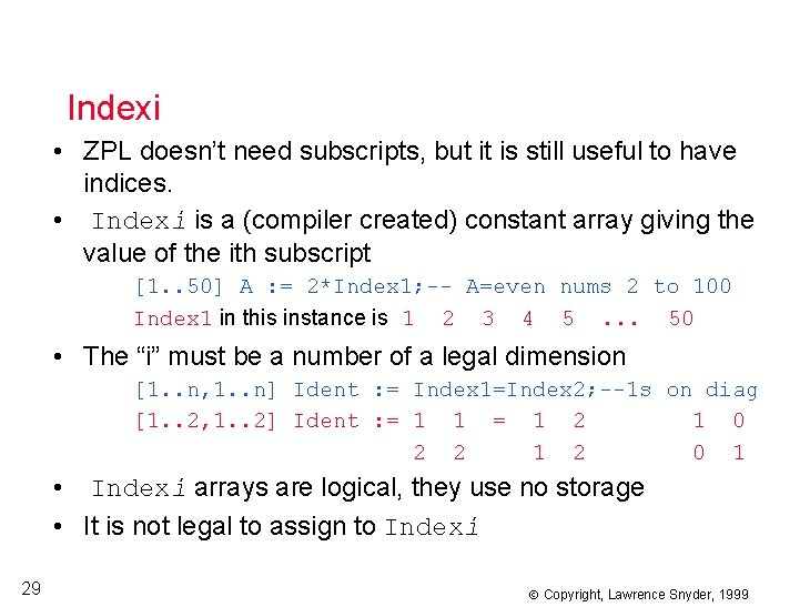
Indexi • ZPL doesn’t need subscripts, but it is still useful to have indices. • Indexi is a (compiler created) constant array giving the value of the ith subscript [1. . 50] A : = 2*Index 1; -- A=even nums 2 to 100 Index 1 in this instance is 1 2 3 4 5. . . 50 • The “i” must be a number of a legal dimension [1. . n, 1. . n] Ident : = Index 1=Index 2; --1 s on diag [1. . 2, 1. . 2] Ident : = 1 1 = 1 2 1 0 2 2 1 2 0 1 • Indexi arrays are logical, they use no storage • It is not legal to assign to Indexi 29 Copyright, Lawrence Snyder, 1999

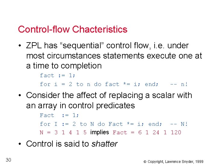
Control-flow Chacteristics • ZPL has “sequential” control flow, i. e. under most circumstances statements execute one at a time to completion fact : = 1; for i = 2 to n do fact *= i; end; -- n! • Consider the affect of replacing a scalar with an array in control predicates Fact : = 1; for I : = 2 to N do Fact *= i; end; -- N! N = 3 1 4 1 5 implies Fact = 6 1 24 1 120 • Control is said to shatter 30 Copyright, Lawrence Snyder, 1999

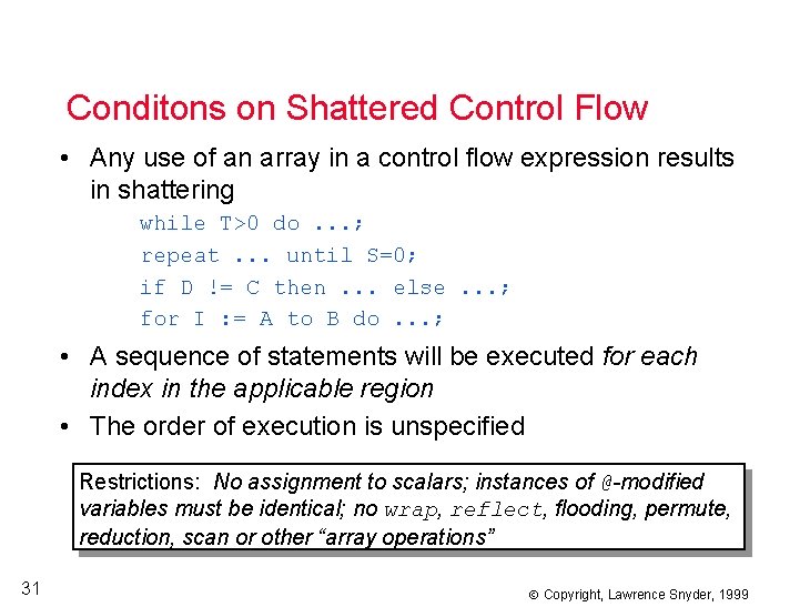
Conditons on Shattered Control Flow • Any use of an array in a control flow expression results in shattering while T>0 do. . . ; repeat. . . until S=0; if D != C then. . . else. . . ; for I : = A to B do. . . ; • A sequence of statements will be executed for each index in the applicable region • The order of execution is unspecified Restrictions: No assignment to scalars; instances of @-modified variables must be identical; no wrap, reflect, flooding, permute, reduction, scan or other “array operations” 31 Copyright, Lawrence Snyder, 1999

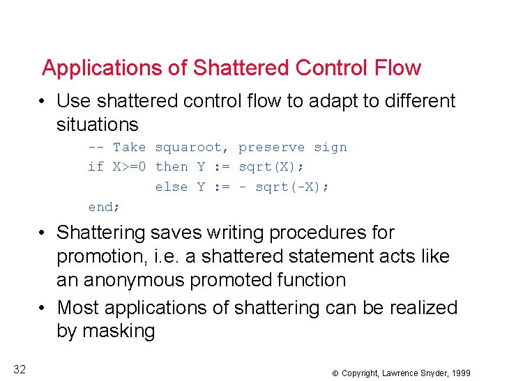
Applications of Shattered Control Flow • Use shattered control flow to adapt to different situations -- Take squaroot, preserve sign if X>=0 then Y : = sqrt(X); else Y : = - sqrt(-X); end; • Shattering saves writing procedures for promotion, i. e. a shattered statement acts like an anonymous promoted function • Most applications of shattering can be realized by masking 32 Copyright, Lawrence Snyder, 1999

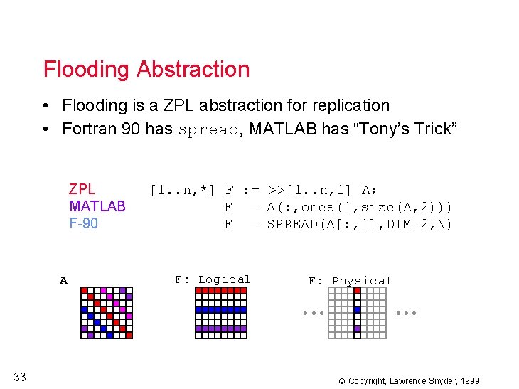
Flooding Abstraction • Flooding is a ZPL abstraction for replication • Fortran 90 has spread, MATLAB has “Tony’s Trick” ZPL MATLAB F-90 A [1. . n, *] F : = >>[1. . n, 1] A; F = A(: , ones(1, size(A, 2))) F = SPREAD(A[: , 1], DIM=2, N) F: Logical F: Physical • • • 33 • • • Copyright, Lawrence Snyder, 1999

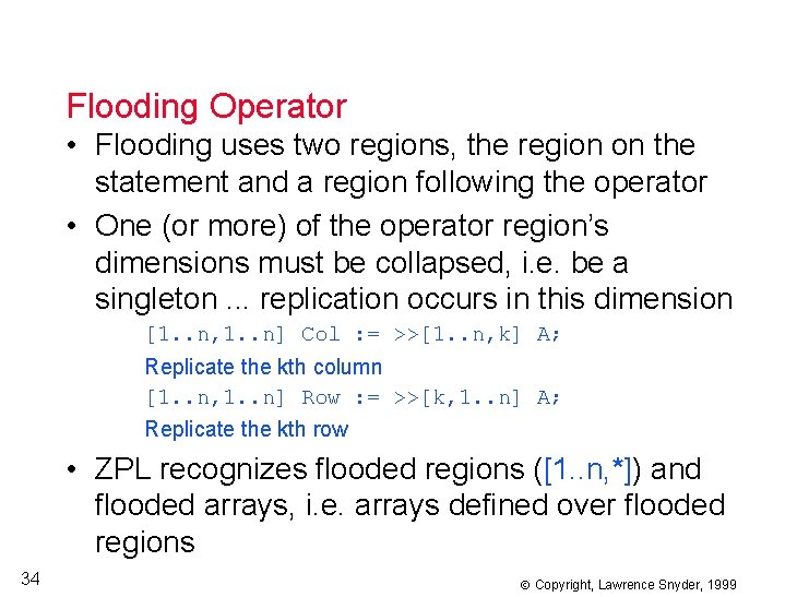
Flooding Operator • Flooding uses two regions, the region on the statement and a region following the operator • One (or more) of the operator region’s dimensions must be collapsed, i. e. be a singleton. . . replication occurs in this dimension [1. . n, 1. . n] Col : = >>[1. . n, k] A; Replicate the kth column [1. . n, 1. . n] Row : = >>[k, 1. . n] A; Replicate the kth row • ZPL recognizes flooded regions ([1. . n, *]) and flooded arrays, i. e. arrays defined over flooded regions 34 Copyright, Lawrence Snyder, 1999

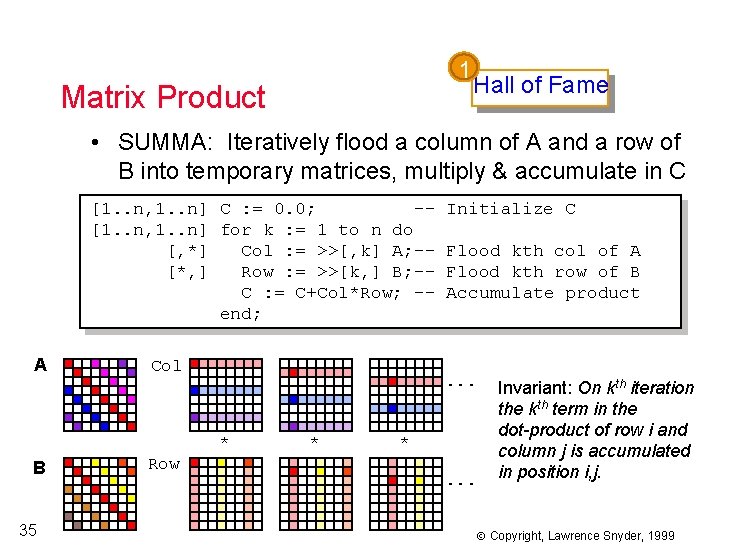
1 Matrix Product Hall of Fame • SUMMA: Iteratively flood a column of A and a row of B into temporary matrices, multiply & accumulate in C [1. . n, 1. . n] C : = 0. 0; -[1. . n, 1. . n] for k : = 1 to n do [, *] Col : = >>[, k] A; -[*, ] Row : = >>[k, ] B; -C : = C+Col*Row; -end; A Col 35 Row Flood kth col of A Flood kth row of B Accumulate product . . . * B Initialize C * *. . . Invariant: On kth iteration the kth term in the dot-product of row i and column j is accumulated in position i, j. Copyright, Lawrence Snyder, 1999

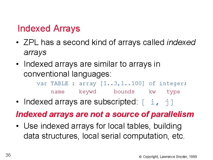
Indexed Arrays • ZPL has a second kind of arrays called indexed arrays • Indexed arrays are similar to arrays in conventional languages: var TABLE : array [1. . 3, 1. . 100] of integer; name keywd bounds kw type • Indexed arrays are subscripted: [ i, j] Indexed arrays are not a source of parallelism • Use indexed arrays for local tables, building data structures, local serial computation, etc. 36 Copyright, Lawrence Snyder, 1999

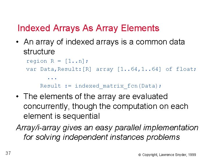
Indexed Arrays As Array Elements • An array of indexed arrays is a common data structure region R = [1. . n]; var Data, Result: [R] array [1. . 64, 1. . 64] of float; . . . Result : = indexed_matrix_fcn(Data); • The elements of the array are evaluated concurrently, though the computation on each element is sequential Array/i-array gives an easy parallel implementation for solving independent instances problems 37 Copyright, Lawrence Snyder, 1999

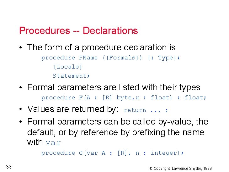
Procedures -- Declarations • The form of a procedure declaration is procedure PName ({Formals}) {: Type}; {Locals} Statement; • Formal parameters are listed with their types procedure F(A : [R] byte, x : float) : float; • Values are returned by: return. . . ; • Formal parameters can be called by-value, the default, or by-reference by prefixing the name with var procedure G(var A : [R], n : integer); 38 Copyright, Lawrence Snyder, 1999

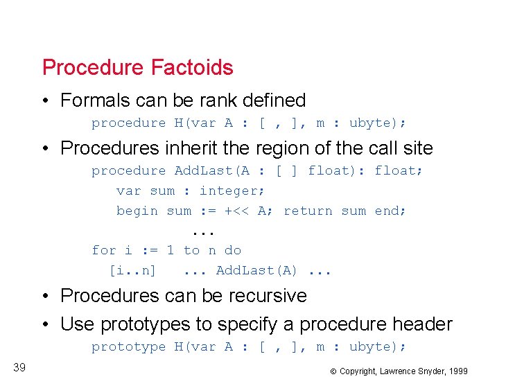
Procedure Factoids • Formals can be rank defined procedure H(var A : [ , ], m : ubyte); • Procedures inherit the region of the call site procedure Add. Last(A : [ ] float): float; var sum : integer; begin sum : = +<< A; return sum end; . . . for i : = 1 to n do [i. . n]. . . Add. Last(A). . . • Procedures can be recursive • Use prototypes to specify a procedure header prototype H(var A : [ , ], m : ubyte); 39 Copyright, Lawrence Snyder, 1999

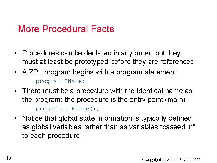
More Procedural Facts • Procedures can be declared in any order, but they must at least be prototyped before they are referenced • A ZPL program begins with a program statement program PName; • There must be a procedure with the identical name as the program; the procedure is the entry point (main) procedure PName(); • Notice that global state information is typically defined as global variables rather than as variables “passed in” to each procedure 40 Copyright, Lawrence Snyder, 1999

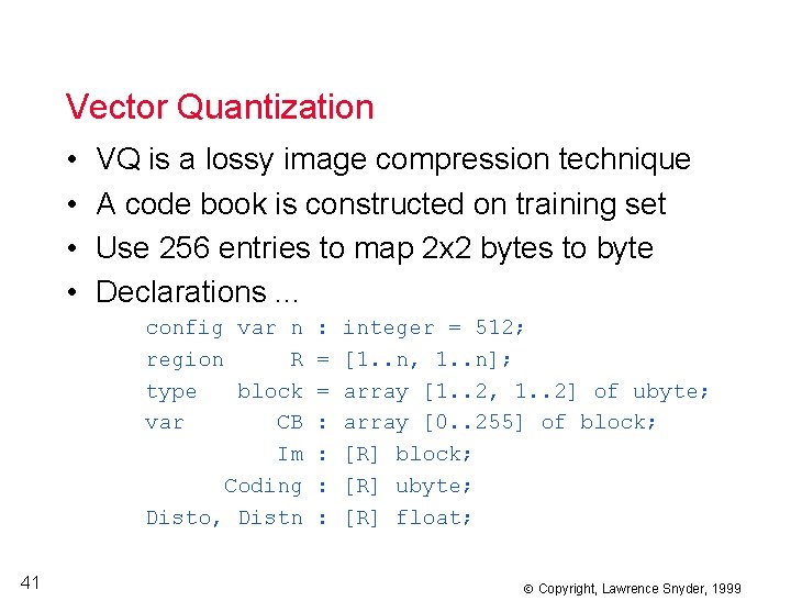
Vector Quantization • • VQ is a lossy image compression technique A code book is constructed on training set Use 256 entries to map 2 x 2 bytes to byte Declarations. . . config var n : integer = 512; region R = [1. . n, 1. . n]; type block = array [1. . 2, 1. . 2] of ubyte; var CB : array [0. . 255] of block; Im : [R] block; Coding : [R] ubyte; Disto, Distn : [R] float; 41 Copyright, Lawrence Snyder, 1999

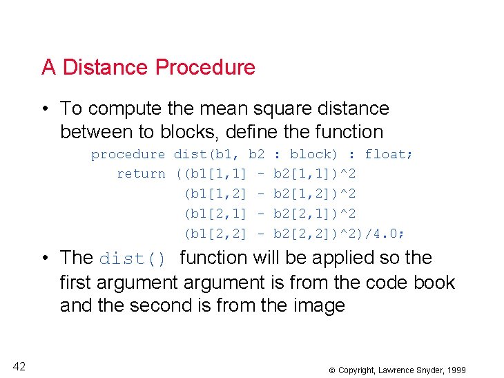
A Distance Procedure • To compute the mean square distance between to blocks, define the function procedure dist(b 1, b 2 return ((b 1[1, 1] (b 1[1, 2] (b 1[2, 1] (b 1[2, 2] - : block) : float; b 2[1, 1])^2 b 2[1, 2])^2 b 2[2, 1])^2 b 2[2, 2])^2)/4. 0; • The dist() function will be applied so the first argument is from the code book and the second is from the image 42 Copyright, Lawrence Snyder, 1999

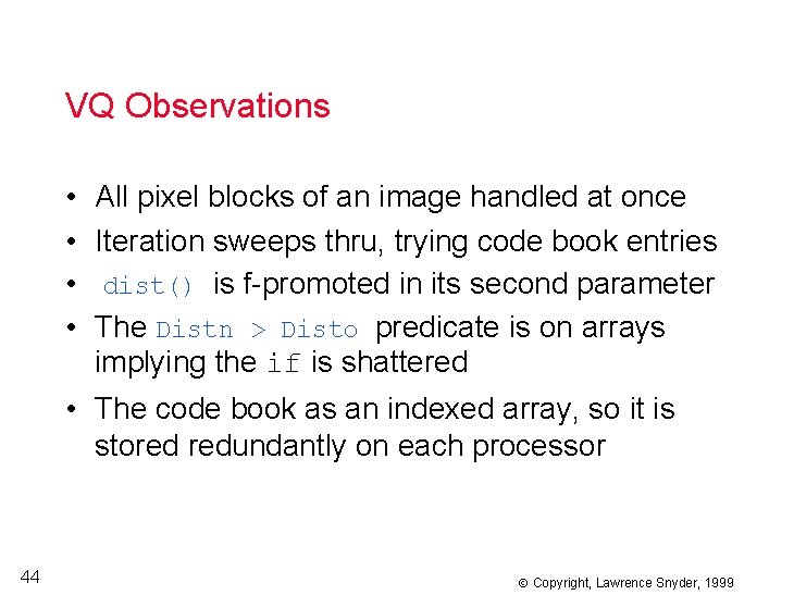
VQ Compression Loop • Assume code book is input 43 [R] repeat -- Imput next image, blocked into Im Disto : = dist(CB[0], Im); --Init w/dist entry 1 Coding : = 0; --Set coding to 1 st for i : = 1 to 255 do --Sweep thru code bk Distn : = dist(CB[i], Im); --dist to ith entry if Disto > Distn then --Is new dist less? Disto : = Distn; -- Y, update distance Coding : = i; -- record the best end; -- Output the compressed image in Coding until no_more_images; Copyright, Lawrence Snyder, 1999

VQ Observations • • All pixel blocks of an image handled at once Iteration sweeps thru, trying code book entries dist() is f-promoted in its second parameter The Distn > Disto predicate is on arrays implying the if is shattered • The code book as an indexed array, so it is stored redundantly on each processor 44 Copyright, Lawrence Snyder, 1999

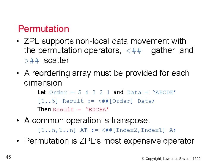
Permutation • ZPL supports non-local data movement with the permutation operators, <## gather and >## scatter • A reordering array must be provided for each dimension Let Order = 5 4 3 2 1 and Data = ‘ABCDE’ [1. . 5] Result : = <##[Order] Data; Then Result = ‘EDCBA’ • A common operation is transpose: [1. . n, 1. . n] AT : = <##[Index 2, Index 1] A; • Permutation is ZPL’s most expensive operator 45 Copyright, Lawrence Snyder, 1999

Summary • ZPL is a new language designed to simplify programming scientific computations • Most of the language structures have been introduced, but much detail remains. . . see the ZPL Programmer’s Guide for specifics • Techniques for finding a solution have been emphasized so far. . . the next topic is techniques for finding fast, parallel solutions 46 Copyright, Lawrence Snyder, 1999