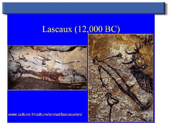
Znanstvena vizualizacija Visualizacija raunalnika grafika znanost Visualization brings

Znanstvena vizualizacija

Visualizacija, računalniška grafika, znanost Visualization brings together two disparate fields, the traditional sciences (like physics, chemistry, biology, for example) and computer graphics

Cilji vizualizacije • Comparing: images, positions, data sets, subsets of data. • Distinguishing: importance, objects, activities, range of value. • Indicating directions: orientations, order, direction of flow. • Locating: position relative to axis, object, map. • Relating: concepts, e. g. value and direction, position and shape, temperature and velocity, object type and value. • Representing values: numeric value of data. • Revealing objects: exposing, highlighting, bringing to the front, making visible, enhancing visibility.

Malo zgodovine

Ena od definicij • The broad class of computer graphic and imaging techniques used to create visual representations of data. • Wolff and Yaeger, Visualization of Natural Phenomena, ELOS, Springer-Verlag, 1993

Kaj je znanstvena vizualizacija? • the mapping of data and/or information to images to gain or present understanding and insight • the visual analysis of scientific data. It transforms the numeric representation into a geometric (image) representation, enabling a scientist, engineer, or mathematician to observe his simulated or measured data • Scientific Visualization encompasses and unifies the fields of computer graphics, image processing, computer vision, computer-aided design, signal processing, and human-computer interaction • Scientific Visualization is a set of software tools coupled with a powerful 3 D graphical computing environment that allows any geometric object or concept to be visualized by anyone. The software provides an easy to use interface for the user. The hardware must be able to manipulate complex, geometricallydescribed, 3 D environments in motion, color, and with any level of “realism” called for to better communicate the essence of the computation (in foreword of An Introductory Guide to Scientific Visualization. R. A. Earnshaw & N. Wiseman, Springer-Verlag, 1992) • Sci. Vi, Sci. Viz, Sci. Vis, SV, . . .

Zakaj znanstvena vizualizacija? • “The purpose of computing is insight, not numbers” Richard Hamming (1962) • “Maintain a Healthy Skepticism: Never believe the results of your calculations. Always look for errors, limitations, unnatural constraints, inaccurate inputs, and places where algorithms break down. Nothing works until it is tested, and it probably does not really work even then. This skepticism should help avoid embarrassing situations, such as occur when a neat physical explanation is painstakingly developed for a computational blunder. ” E. S. Oran & J. P. Boris (1987) • “In decreasing order of importance, scientific visualization: - shows you where you are screwing up - allows discoveries - is useful for show-and-tell” J. J. O’Brien (1993)

Aplikacije

Visualisation for Education

Visualisation for Architecture

Visualisation in Interface Design

Visualising Group Work

Visualising Complexity

Scientific Visualization in the Geosciences

Visualization for Biological and Physical Scientists

Medical/Bioinformatics

NLM Visible Human Project • An outgrowth of the NLM's 1986 Long-Range Plan. • Creating a complete, anatomically detailed, three-dimensional representations of the male and female human body. • The current phase of the project is collecting transverse CT, MRI and cryosection images of representative male and female cadavers at one millimeter intervals.

Visualising Non-Physical Systems Time Days in May Frequencies of Each Event Over Time Event Class (Vulnerabilities & Attacks) User can click on frequency bar to see which hosts were the targets of the events

Visualising Non-existing Systems Eg Visual Interactive Simulation Systems Modelling

Visualization in Computational Science • Computational Science refers to the knowledge and techniques required to perform computer simulations and tackling computationally intensive problems. • Main goal of Computational Science: – To understand the workings of nature • Steps – Observations, Physical Model, Mathematical Model, Numerical Model, Simulation and Analysis

The Research Triangle Theoretical Science Experimental Science Computational Science

Domene raziskovanja Experimentalist’s Domain Observations Physical Model Theorist’s Domain Computational Scientist’s Domain Mathematical Model Numerical Model Simulation & Analysis

Computational Cycle Research Summarize Program Analyze Simulate Compute

Analysis Cycle Summarize Simulate Raw Data Playback Filter Data Mapping Geometric Primitive Images Renderer

Od resničnosti do slike Reality Experimental Model Mathematical Model Data Visualization Picture Better Data

Zakaj vizualizacija podatkov? A Picture is worth a Million Bytes 34 4 F D 2 73 89 2 E 12 90 E 1 45 FF FF 6 A B 4 78 54 23 D 2 AA 38 90 36 87 54 DD C 2 FF 89 00 Data 76 Information

Proces znanstvene vizualizacije Summarize Data Source Filter Data Playback Data Images Render Mapping Geometric Primitives
 • Simulated (computed)")
Types of Source Data • Measured (sensed, observed, experimental) • Simulated (computed)

Predstavitev podatkov za vizualizacijo Computational Methods Measurement Modelling Transform Data Map Display

Possible Research • • Visualization of time-dependent motion Change of topology Interactive feature extraction Interactive exploration Use of force feedback in visualization Handling of Multi-Gigabyte datasets Exploration of high-dimensional spaces

Types of Scientific Visualization • I See – – interactive exploratory softcopy display minimal contextual information – – interactive exploratory softcopy display more context/explanation needed – – – presentation usually not interactive not exploratory hardcopy display lots of context/explanation needed • We See • They See

Data and Scientific Visualisation
")
Measured Data – LIDAR (Light Detection and Ranging)
![Primeri iz programa Mathematica Parametric. Plot 3 D[{t*Cos[t^2], t*Sin[t^2], t}, {t, 0, 2 Pi},](http://slidetodoc.com/presentation_image_h2/866ada1182d33a686aaab8db1b8aa76a/image-38.jpg "Primeri iz programa Mathematica Parametric. Plot 3 D[{t*Cos[t^2], t*Sin[t^2], t}, {t, 0, 2 Pi},")
Primeri iz programa Mathematica Parametric. Plot 3 D[{t*Cos[t^2], t*Sin[t^2], t}, {t, 0, 2 Pi}, Plot. Points->200] Parametric. Plot 3 D[{Cos[u] Cos[v], Sin[v]}, {u, 0, 2 Pi}, {v, -Pi/2, Pi/2}]
![Primeri iz programa Mathematica f[x_, y_]=(x^2 -3)y^2; cpone=Contour. Plot[f[x, y], {x, -3, 3}, {y,](http://slidetodoc.com/presentation_image_h2/866ada1182d33a686aaab8db1b8aa76a/image-39.jpg "Primeri iz programa Mathematica f[x_, y_]=(x^2 -3)y^2; cpone=Contour. Plot[f[x, y], {x, -3, 3}, {y,")
Primeri iz programa Mathematica f[x_, y_]=(x^2 -3)y^2; cpone=Contour. Plot[f[x, y], {x, -3, 3}, {y, -1, 1}, Display. Function->Identity]; cptwo=Contour. Plot[f[x, y], {x, -3, 3}, {y, -1, 1}, Plot 3 D[Cos[Sin[x]+Cos[y]], Contour. Style->Gray. Level[. 7], {x, 0, 2 Pi}, {y, -Pi, Pi}] Contour. Shading->False, Display. Function->Identity]; Show[Graphics. Array[{cpone, cptwo}]]

Kaj je podatek?
")
Polja (fields)
")
Mreže in podatki (mesh and data)

Drugi tipi 3 D podatkov
 – 2 D, 3 D, 4")
Dimenzije in tipi podatkov • domain (independent variables) – 2 D, 3 D, 4 D, etc. – if the data points are not connected: scattered – if the domain is gridded: • rectilinear (uniform [regular] or non-uniform [irregular]) – cubes: with data points at vertices, on faces, or in the center • curvilinear – distorted cubes, but 6 -connectivity at nodes, analogy is a distorted sponge • unstructured – 2 D - triangles – 3 D – tetrahedra, prisms, pyramids, or hexahedra • range (dependent variables) – scalar (pressure, density, temperature, voltage, height, salinity) – vector (velocity, current, gradient, etc. ) – tensor (stress, strain, etc. )

Grids

Uniform Data

Grids

Curvilinear Data

Unstructured Data

Unstructured Data

Common steps in volume visualization algorithms • • • data acquisition slice processing dataset reconstruction dataset classification mapping into primitives

Tehnike za 3 D skalarne veličine

Klasifikacija podatkov • • most difficult task choose threshold if SF algorithm choose color and opacity for range of data values if DVR other factors – user’s knowledge of the material (data) being visualized • if the f(x) are density values and you know bone has a density of 0. 8 and you want to see bone, you set the opacity of f(x)=0. 8 to 1. 0 – the location of the classified elements in the volume • often want outer layers more transparent, thus element position is factored into the formula – the material occupancy of the element • When the data values are changing slowly, only a narrow range of values is acceptable as the isovalue surface. When the data values are changing rapidly, a wide range of values is acceptable as the isovalue surface.

How to turn data into an image • Ultimately you turn on a discrete point on the computer screen or you put a finite quantity of colored material on some material or …wet chemistry. • You have to make a lot of choices in how you want that done. • The process can be divided in mathematical steps, scientific steps, and engineering steps.

Klasifikacija tehnik vizualizacije • Glyph techniques – use symbols to represent values or states within a field of information. • Surface Methods – extracts polygonal versions of calculated components. • Direct Volume Rendering – generates a rendered image of the volume where volume elements are projected directly onto the image plane.

Metode vizualizacije prostornin • Cutting Planes • Isosurfaces • Direct Volume Rendering
")
Metode vizualizacije prostornin The fundamental algorithms are of two types: direct volume rendering (DVR) algorithms and surface-fitting (SF) algorithms. DVR methods map elements directly into screen space without using geometric primitives as an intermediate representation. DVR methods are especially good for datasets with amorphous features such as clouds, fluids, and gases. A disadvantage is that the entire dataset must be traversed for each rendered image. Sometimes a low resolution image is quickly created to check it and then refined. The process of increasing image resolution and quality is called "progressive refinement". SF methods are also called feature-extraction or iso-surfacing and fit planar polygons or surface patches to constant-value contour surfaces. SF methods are usually faster than DVR methods since they traverse the dataset once, for a given threshold value, to obtain the surface and then conventional rendering methods (which may be in hardware) are used to produce the images. New views of the surface can be quickly generated. Using a new threshold is time consuming since the original dataset must be traversed again.

Cutting Planes

3 D Wireframe Isosurface

3 D Polygonal Isosurface

Isosurface + Contour Plane

Isosurfaces of Medical Data
 – The three steps to isosurface construction are: • detect surface(s)")
Konstrukcija Izo-površin (isosurfaces) – The three steps to isosurface construction are: • detect surface(s) • fit geometric primitives to the detected surface(s) • render surface – two methods for fitting geometric primitives: • contour connection methods • voxel intersection methods – dividing cubes – marching cubes – Marching Cubes works by classifying the eight nodes of a voxel as being greater-than or less-than a threshold. These eight bits are used as an index into an edge intersection table. Linear interpolation is used to determine edgeintersection location and triangles are fitted to the edges. The triangles and the surface normals at vertices are added to a linked list for rendering.

Voksli in celice – The amount of structure in the dataset usually determines which volume visualization algorithm will create the most informative images. Voxels and Cells – Volumes of data can be treated as either an array of volume elements (voxels) or an array of cells. • voxel - the area around a data point • cell - views volume as a collection of hexahedra whose corners are the data points Almost every volume visualization algorithm requires resampling which requires interpolation (or reconstruction).
 • image-order - for each pixel see what objects (elements) project onto")
Prečkanja (traversals) • image-order - for each pixel see what objects (elements) project onto the pixel (remember, a pixel covers an area on the screen). • object-order - for each object (element) see where it intersects the image plane – can progress front-to-back (saves some computation potentially), or – back-to-front (can see scene evolve)

Fotorealizem Photorealism is a hotly debated issue in DVR. The issue is should objects look like they are made from “real” material? The problem is that plausible objects may be misleading, but nonplausible may be hard to interpret. No consensus exists.

Scalar Data in 3 D Examples: • Temperatures in a room • Molecular potentials Techniques: • Colored dots (“point cloud”) • Cutting plane • Isosurfaces

3 D Jittered Point Cloud

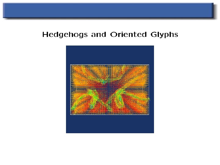
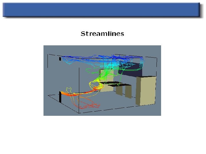
Vector Data in 3 D Examples: • 3 D flow field Techniques: • Arrows (“vector cloud”) • Streamlines

3 D Flow Field
 Glyph techniques – use symbols to represent values or")
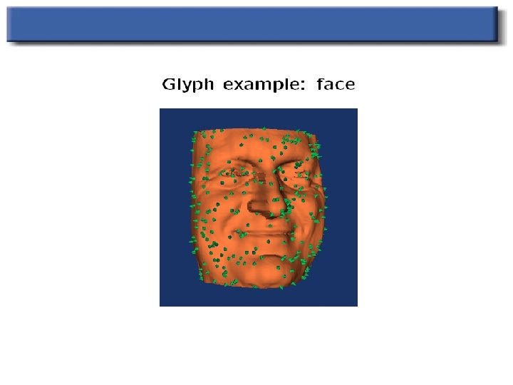
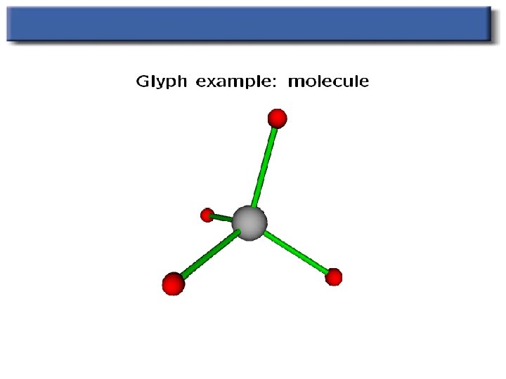
Tehnike s figurami (Glyph Techniques) Glyph techniques – use symbols to represent values or states within a field of information.
")
Figure (glyphs)
")
Figure (Glyphs)

Še o algoritmih

Skalarni algoritmi
")
Barvne preslikave in izo površine (color maps and isosurfaces)

Primeri barvnih preslikav
 Transfer function maps data/colours Non-linear transfer functions enhance ranges of")
Barvne preslikave (Colour Maps) Transfer function maps data/colours Non-linear transfer functions enhance ranges of data High contrast centre High contrast extremes obfuscation R G B Colour Index

Vektorski algoritmi

FEM and 3 D data visualization Visualized with Amira Vector Fields: • illuminated field lines (courtesy TGS)

Heat Convection between Two Plates Data, courtesy David Yeun 2573 dataset 643 subsampling Heat flow between two plates at constant temperature

Tenzorski algoritmi
 z = f(x, y) f = f(x, y, z)")
Dimenzije vizualizacije y = f(x) z = f(x, y) f = f(x, y, z) Graphs/Histograms Contours Volume visualisation Charts False Colour Isosurfaces
, u(x, y, z) Price p(t) Height h(x, y)")
Dimenzije atributov • Scalar Temperature u(t), u(x, y, z) Price p(t) Height h(x, y) • Vector eg. Velocity (u, v), (u, v, w) Share Price and Volume p(t), V(t) Gradient of a Scalar • Tensor eg. Stress and Strain u(x, y) = (du/dx , du/dy) a 11, a 12, a 13 a 21, a 22, a 23 a 31, a 32 , a 33

One Dimensional Visualisation • Ancient Technique • Plots, Graphs, Bar charts etc. • Log. /Linear Scales • Join data points • Label Axes

Linear Graphing Techniques Interpolation Linear - fast, simple Linear and Non-linear Non-Linear - eg polynormal, Spline Used where clear trend exits Can distort data

Two Dimensional Visualisation Cells Grids Unstructured
 = constant")
2 D Visualizations • Contour Lines - f(x, y) = constant

2 D Color Interpolation

2 D Contours

Same Data, Different Geometrization

2 D Visualization • Vector Fields – Hedgehogs – Streamlines

2 D Data Techniques Kriging Technique for inferring points on a 2 D plane Data points are weighted according to their proximity to the interpolant

2 D Data Techniques Contouring Data: Contours are lines of constant function value Contour, path (x, y) so that f(x, y) = constant Examples: c = 100 m above sea level. C is a constant intensity in MRI scan. C is a constant ozone concentration.
 • Scan")
2 D Data Techniques Contouring Select height (e. g. c = 5) • Scan cells until an edge crossing c is found • Find location of crossing with inverse linear interpolation. • Locate exit edge • Mark checked edges • move to next cell (exit cell becomes entrance edge) 0 1 1 3 2 1 3 6 6 3 3 7 9 7 3 3 8 9 6 4 2 7 8 6 2 1 2 3 4 3

2 D Data Techniques Contouring 1 5 2 6 3 7 Marching Squares 4 0 0 1 1 3 2 1 3 6 6 3 3 7 9 7 3 3 8 9 6 4 2 7 8 6 2 1 2 3 4 3
 defines a planar polygon. Coordinates of vertices x; y; z")
Surface Modelling Each (triangular) defines a planar polygon. Coordinates of vertices x; y; z Calculate polygon normal Render with a lighting model Colour may indicate height or be spurious! Looks pretty Difficult to obtain quantitative information
 Architectural Walk-throughs")
Three Dimensional Visualisation Used especially in Medical Applications Simulations (eg flight training) Architectural Walk-throughs

Example 3 D Visualisation

Example 3 D Visualisation

Zaključki • Emerging Field of computing • Needs high processing and graphics capabilities • Wide ranging application • No dominant standards and norms (exploratory area) • Large design input • Potential to obfuscate as well as enlighten • Needs to reflect needs of end users (not technology for its own sake)
 – Isosurface,")
Zaključki • Extract from large datasets more meaningful components (called data extracts) – Isosurface, streamlines, streaklines, vector field topology, vortex tubes, cracks, fault lines, etc. – Sedimentation layers, free-surfaces, edge and surface extraction • Render this data with comprehension in mind, as opposed to visual realism

Zaključki • Strike balance between – High- resolution versus interactive speed • How to • Time-dependent visualization • Describe and view change of data topology – Vector and scalar fields – Tensor fields (i. e. , rate of strain tensor) • How to navigate a Terabyte dataset?
- Slides: 108