Young Lee Jayant Kalagnanam Jane Snowdon Estepan Meliksetian
- Slides: 12

Young Lee, Jayant Kalagnanam, Jane Snowdon, Estepan Meliksetian, Lianjun An, Pawan Chowdhary, Chandra Reddy, Fei Liu, Paul Nevil, Raya Horesh September 17, 2010 Smarter Buildings: A Statistical Modeling Strategy for Energy Efficiency of Buildings © 2010 IBM Corporation

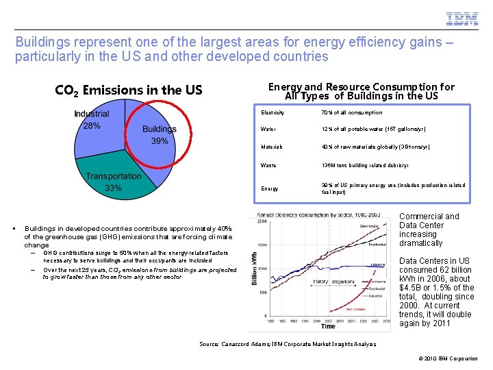
Buildings represent one of the largest areas for energy efficiency gains – particularly in the US and other developed countries CO 2 Emissions in the US § Buildings in developed countries contribute approximately 40% of the greenhouse gas (GHG) emissions that are forcing climate change – GHG contributions surge to 50% when all the energy-related factors necessary to serve buildings and their occupants are included – Over the next 25 years, CO 2 emissions from buildings are projected to grow faster than those from any other sector Energy and Resource Consumption for All Types of Buildings in the US Electricity 70% of all consumption Water 12% of all potable water (15 T gallons/yr) Materials 40% of raw materials globally (3 B tons/yr) Waste 136 M tons building related debris/yr Energy 39% of US primary energy use (includes production-related fuel input) Commercial and Data Center increasing dramatically Data Centers in US consumed 62 billion k. Wh in 2006, about $4. 5 B or 1. 5% of the total, doubling since 2000. At current trends, it will double again by 2011 Source: Canaccord Adams; IBM Corporate Market Insights Analysis, EPA Report to Congress, August 2, 2007 © 2010 IBM Corporation

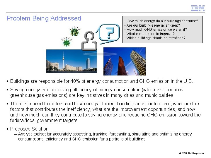
Problem Being Addressed - How much energy do our buildings consume? - Are our buildings energy efficient? - How much GHG emission do we emit? - What can be done to improve? - Which buildings should be retrofitted? § Buildings are responsible for 40% of energy consumption and GHG emission in the U. S. § Saving energy and improving efficiency of energy consumption (which also reduces greenhouse gas emissions) are key initiatives in many cities and municipalities § There is a need to understand how energy efficient buildings in a portfolio are, what are the factors that contributes the inefficiency, what are the improvement opportunities, and how much can they contribute to saving energy and reducing GHG emission toward the federal/local government targets § Proposed Solution – Analytic toolset for accurately assessing, tracking, forecasting, simulating and optimizing energy consumptions, efficiency and GHG emission for a portfolio of buildings © 2010 IBM Corporation

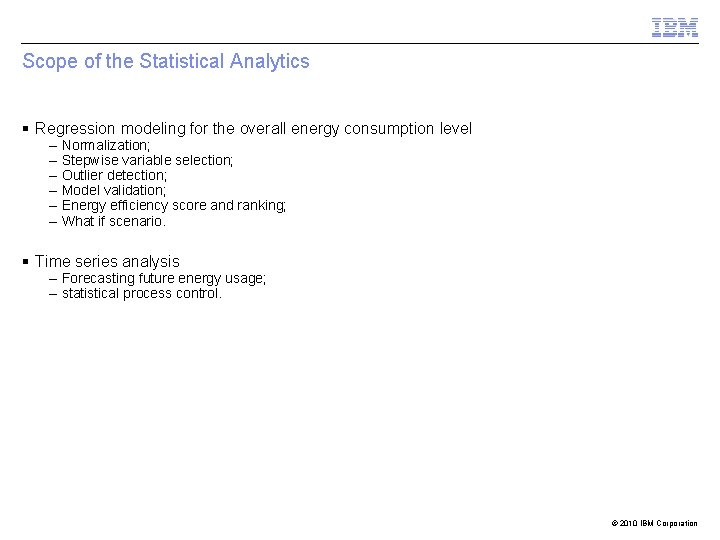
Scope of the Statistical Analytics § Regression modeling for the overall energy consumption level – – – Normalization; Stepwise variable selection; Outlier detection; Model validation; Energy efficiency score and ranking; What if scenario. § Time series analysis – Forecasting future energy usage; – statistical process control. © 2010 IBM Corporation

Regression Model: Overview § The regression model aims at learning the mean level of energy consumptions. – – What predictor variables are influential on the average energy consumption? How much energy do we expect a school to consume? How much energy can we save with retrofit? How does each school perform relatively? § Exploratory analysis suggests we take logarithm transformation of the energy consumption and the GFA. § Thus, in our analysis, the response variable is the average energy consumption over the 5 year period. § Potential predictor variables we consider are – – – – Cooking facility (1/0); Number of computers; Percentage of AC; Number of students; Log(GFA); Number of floors; Year built. © 2010 IBM Corporation

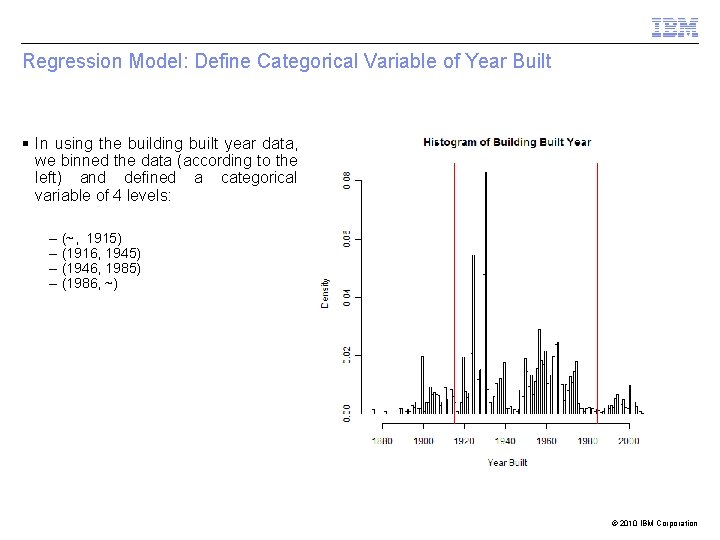
Regression Model: Define Categorical Variable of Year Built § In using the building built year data, we binned the data (according to the left) and defined a categorical variable of 4 levels: – – (~, 1915) (1916, 1945) (1946, 1985) (1986, ~) © 2010 IBM Corporation

Regression Model: Setup and Summary § In the regression model, we select variables by stepwise variable selection procedure. The following variables are selected at the end of the analysis: – – – Log(GFA) PAC YEAR 4 NComputers NStudents NFloors § In the initial fitted model, all observations are included. § We also perform an outlier detection procedure in the analysis. Observations with residuals fall outside 3 sd are treated as outliers and removed from the subsequent analysis. § After removing these outliers, a regression model is refitted. A substantial improvement are observed, and variables being included in the model are: – – – Log(GFA) PAC Year 4 NComputers Cooking NFloors © 2010 IBM Corporation

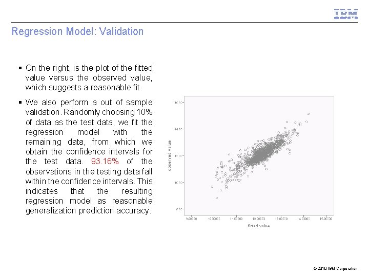
Regression Model: Validation § On the right, is the plot of the fitted value versus the observed value, which suggests a reasonable fit. § We also perform a out of sample validation. Randomly choosing 10% of data as the test data, we fit the regression model with the remaining data, from which we obtain the confidence intervals for the test data. 93. 16% of the observations in the testing data fall within the confidence intervals. This indicates that the resulting regression model as reasonable generalization prediction accuracy. © 2010 IBM Corporation

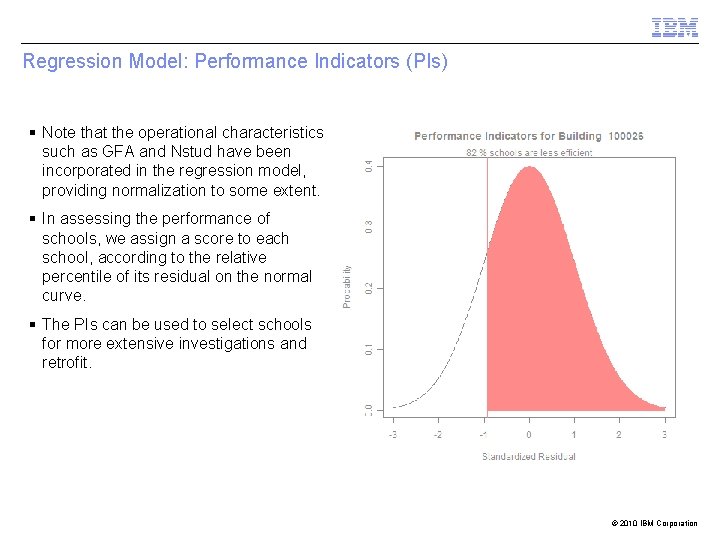
Regression Model: Performance Indicators (PIs) § Note that the operational characteristics such as GFA and Nstud have been incorporated in the regression model, providing normalization to some extent. § In assessing the performance of schools, we assign a score to each school, according to the relative percentile of its residual on the normal curve. § The PIs can be used to select schools for more extensive investigations and retrofit. © 2010 IBM Corporation

Time Series Analysis: Overview § The time series analysis aims at understanding the seasonal and temporal trend of the energy consumption. – Forecasting future energy usage given weather forecasting information. – Statistical process control and monitoring. § We first normalize the history data of each building according to its mean and standard deviation. § The HDD & CDD are also included as the covariates. § A variety of time series models are considered, and the best model is selected based on BIC. – Simple Exponential smoothing models (simple, Brown’s, Holt’s, Damped-trend, Simple seasonal, winters’ additive, winters’ multiplicative); – ARIMA models. © 2010 IBM Corporation

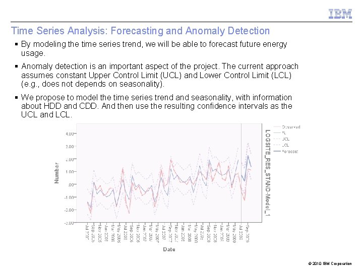
Time Series Analysis: Forecasting and Anomaly Detection § By modeling the time series trend, we will be able to forecast future energy usage. § Anomaly detection is an important aspect of the project. The current approach assumes constant Upper Control Limit (UCL) and Lower Control Limit (LCL) (e. g. , does not depends on seasonality). § We propose to model the time series trend and seasonality, with information about HDD and CDD. And then use the resulting confidence intervals as the UCL and LCL. © 2010 IBM Corporation

Summary § Statistical models can help us to understand the relationship between building energy consumptions and their characteristics. § We can use the regression model to estimate the energy savings from retrofit and what-if scenarios, which would be hard to estimate otherwise. § The performance indicator provides a guideline for further investigation and retrofit. § The time series model can help to forecast and monitor the real time the energy consumption. § The analysis is implemented in the online tracking system and is conducted repeatedly so that the end users can obtain the update to date information promptly. © 2010 IBM Corporation